10 Feb 2020
** This is a study & review of the Homa: A Receiver-Driven Low-Latency Transport Protocol Using Network Priorities paper. I’m not an author.
Homa: A Receiver-Driven Low-Latency Transport Protocol Using Network Priorities
Introduction
- Homa: a new transport protocol designed for small messages in low-latency datacenter environments.
- 99% round trip latencies <= 15 μs for small messages at 80% network load with 10 Gbps link speeds (also improves large messages)
- Priority queues
- Assigns priorities dynamically on receivers
- Integrates the priorities with receiver-driven flow control mechanism similar to pHost, and NDP
- Controlled over-commitment
- Receiver allows a few senders to transmit simultaneously
- Slight over-commitment -> bandwidth efficiency ↑
- Sustain 2-33% higher network loads than qFabric, PIAS, pHost, NDP
- Message-based architecture, not streaming -> reduce head-of-line blocking, 100x over streaming like TCP
- Connectionless -> few connection state in large applications
- No explicit acknowledgements -> reduce overhead for small messages
- At-least-once semantics, not at-most-once
Motivations & Key Ideas
- Low latency hardware popular
- Most of the traffic in datacenter are less than 1000 bytes (70%-80%), aka small messages.
- But existing transport designs cannot achieve lowest possible latency for small messages.
- Challenges & solutions
- Eliminate queuing delays, worst-case: incast
- Potential solution: schedule every packet at a central arbiter, Fastpass.
- Cons: need to wait for scheduling decision, 1.5x RTT.
- Homa: transmit short messages blindly (without considering congestions) to cover the half RTT( to the receiver), RTTBytes = 10KB in 10 Gbps network
- Buffering, inevitable
- Potential solutions: rate control, reserve bandwidth headroom, limit buffer size
- Cons: cannot eliminate penalty of buffering
- Homa: use in-network priorities. Short messages processed before large messages. SPRT (shortest remaining processing time first) policy
- qFabric: too many priority levels for today’s switches. PIAS: assign priorities on sender, limi approximation of SRPT. QJUMP: manual assignment of priorities, inflexible.
- Priorities must be controlled by the receiver, because receiver have more information on the downlink (bandwidth, set of messages…) so that the receiver can best decide priority for incoming packet.
- Receivers must allocate priorities dynamically,
- Large message: priority based on exact set of inbound messages -> eliminates preemption lag.
- Small message: provide guidance (priority) based on recent work-load.
- Receivers must overcommit their downlink in a controlled manner.
- Scheduling transmission with grants from receiver -> multiple grants simultaneously -> sender need time to process -> hurt performance, max load pHost 58%-73%
- Overcommit: allowing small set of senders send simultaneously.
- Sender uses SRPT also
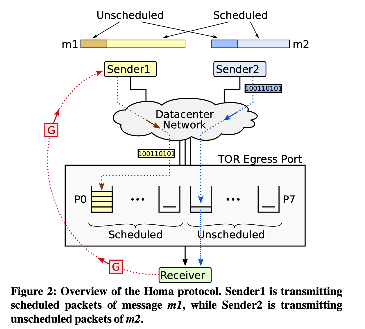
- Unscheduled: RTTBytes, blindly.
- Schedule: wait for receiver response.
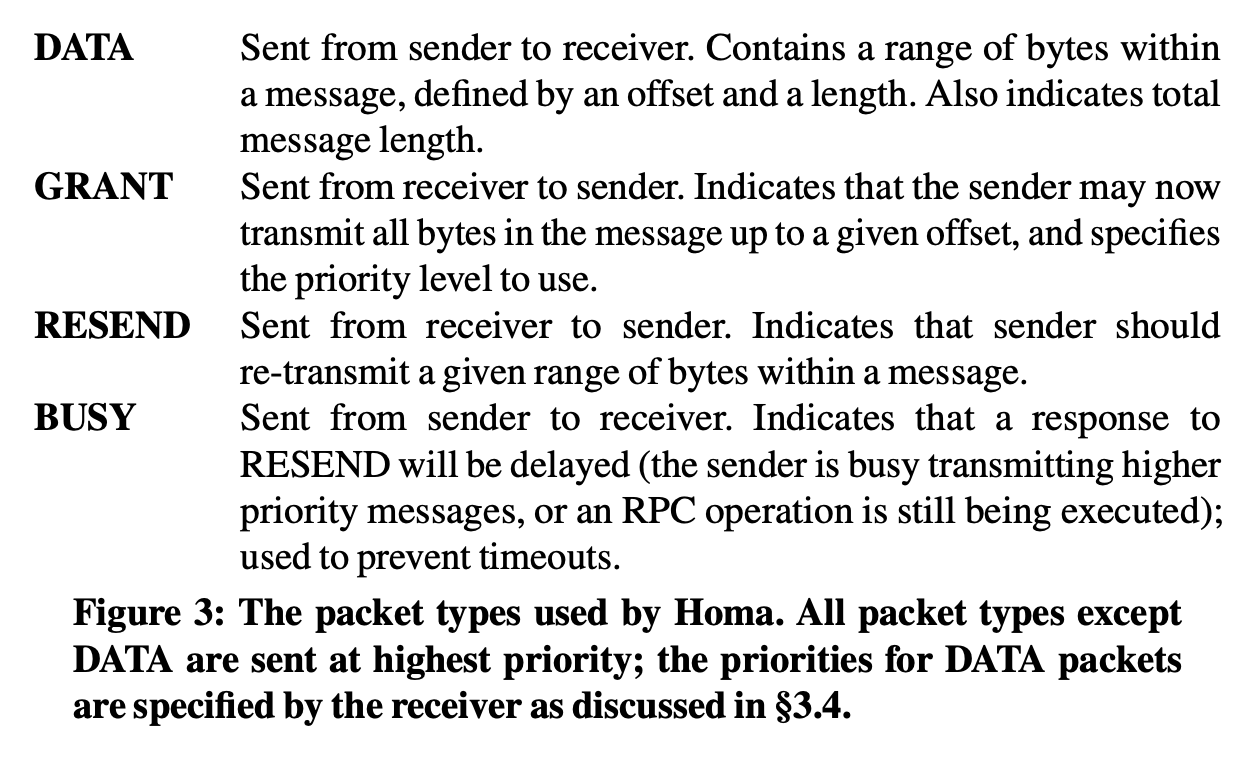
- G: grant packet: acknowledge receipt with priority
Designs
-
-
Priorities
-
Unscheduled packet
- Use recent traffic patterns
- Piggyback on other packets when receiver need to communicate with sender
- $\frac{unscheduled\ bytes}{all\ bytes}$ , for example 80%
- Allocate highest priorities for unscheduled packets (7 out of 8 for 80%).
- Choose cutoffs between unscheduled priorities, so that each priority level is used for an equal amount of unscheduled bytes and shorter messages uses higher priorities.
-
Scheduled packet
- Receiver specify priority and granted bytes in GRANT packet.
- Use low priorities when message amount less than scheduled priorities, reserving higher priorities to avoid preemption lags.
-
Overcommitment
- A receiver grant to more than one sender at a time: take advantage of free bandwidth for unresponsive senders
- If some senders unresponsive: take free bandwidth. If all senders responsive, priority ensures short messages arrive first, and buffering in TOR switch.
- Degree of Overcommitment: max number of active messages at once at a receiver.
- $DoV = #\ of scheduled\ priority\ levels$ , one message per priority level
-
Incast
- Counting outstanding RPCs to detect impending incast, mark new RPCs with special flags, and use lower limit for unscheduled bytes
- Because of Homa’s low latency design, and future deployment of low=latency environments (hardware + software), incast is largely rare
-
Loss Detection
- Lost is rare in Home
- Lost of packets is detected by receiver, send RESEND after timeout identifying first missing bytes range.
Eval
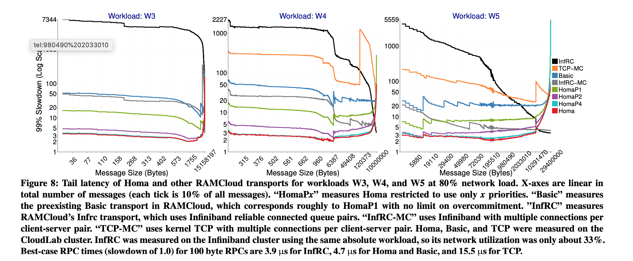
- Great for processing small messages, also performs good with large messages.
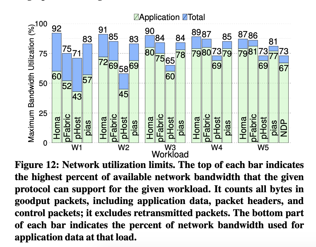
- Network utilization is high
- More comparisons to other protocols, refer to the paper.
Conclusion
∙ It implements discrete messages for remote procedure calls, not byte streams.
∙ It uses in-network priority queues with a hybrid allocation mechanism that approximates SRPT.
∙ It manages most of the protocol from the receiver, not the sender.
∙ It overcommits receiver downlinks in order to maximize throughput at high network loads.
∙ It is connectionless and has no explicit acknowledgments.
10 Feb 2020
** This is a study & review of the ExLL paper. I’m not an author.
ExLL: An Extremely Low-latency Congestion Control for Mobile Cellular Networks
Intro
-
Data latency: devastating effect on applications, such as self-driving cars, autonomous robots, and remote surgery (5G apps)
- TCP sessions often have long delay: bufferfloat: over-buffering problem at bottleneck link because of TCP’s loose congestion control
- More paper confirming bufferfloat is severe in cellular network
Cellular Network Characteristics for Protocol Design:
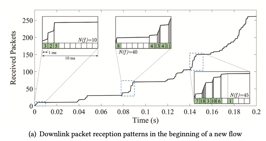
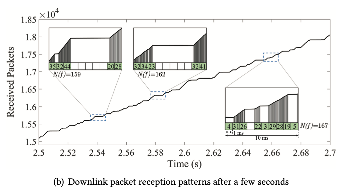
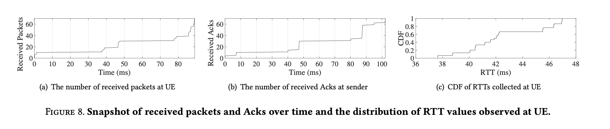
- Downlink Scheduling: the base station (BS) schedules downlink packets towards multiple user equipments (UEs) at 1 ms granularity (a.k.a. transmission time interval, TTI), based on both the signal strength reported by each UE and the current traffic load -> Infer cellular link bandwidth instantly with reception pattern rather than explicitly probing for bandwidth or measuring for a long period of time
- Uplink Scheduling: (the BS needs to grant uplink transmission eligibility for each UE, which happens at a regular interval known as SR (scheduling request) periodicity) Ignoring this periodicity -> underestimate minimum RTT -> CC to run in unrealistic operating conditions.
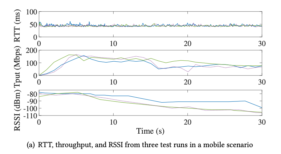
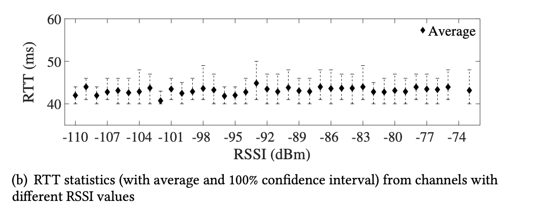
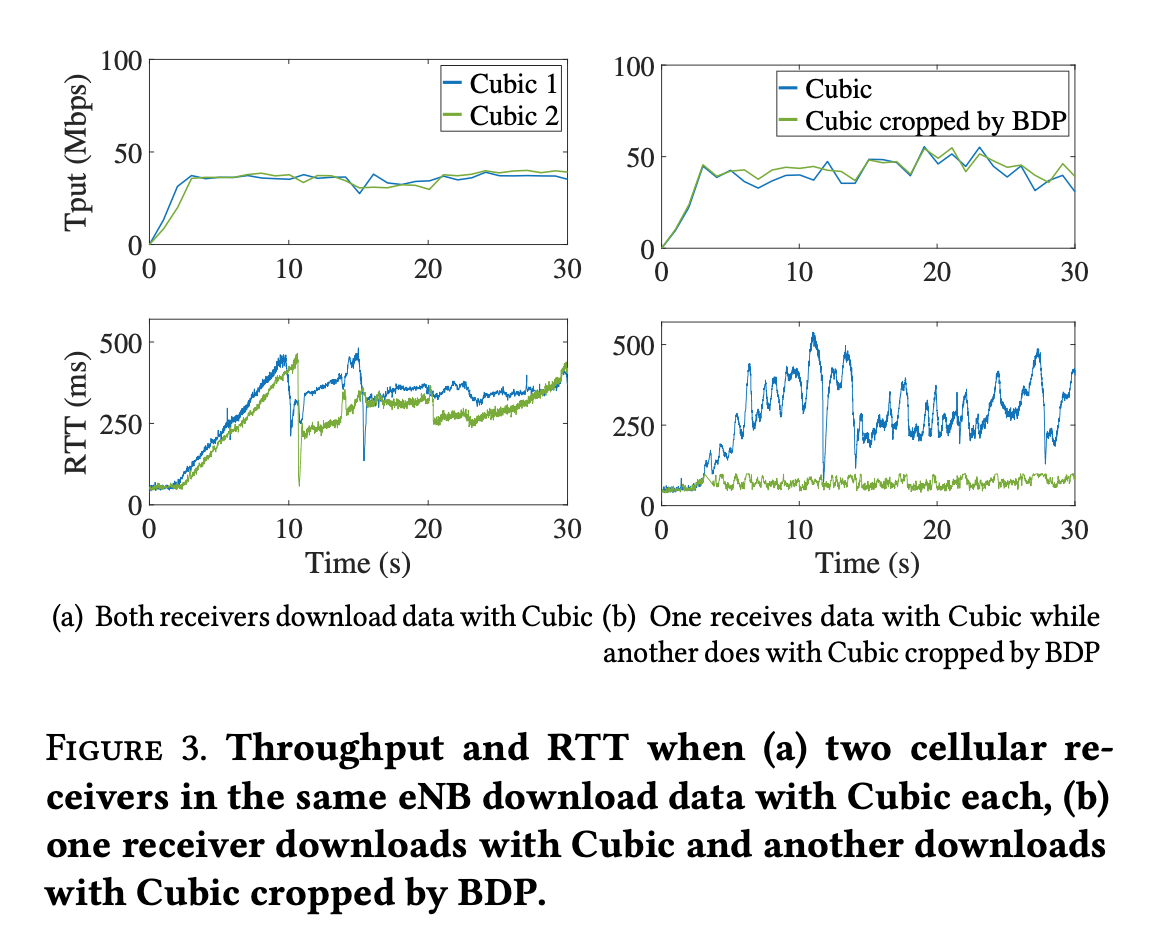
- Minimum RTT is not affected by channel condition between UR and BS (due to adaptive MCS (modulation and coding scheme) selection used in LTE systems, which approximately eliminates MAC-layer retransmissions, but also not affected by other UEs connected to the same BS since per-UE queue is isolated)
Existing Protocols:
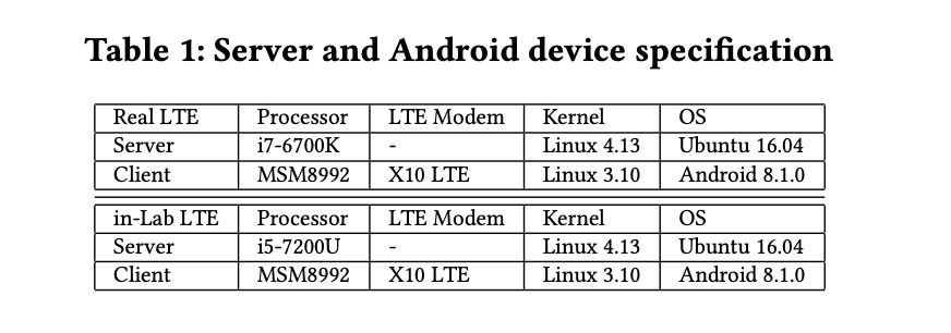
Testing done with Android phones and LTE connections
- Low latency and throughput can’t be achieved together
- ExLL:
- Target: Low latency with high throughput
- Estimations done at UE -> ExLL a receiver-drive CC
- Estimates bandwidth of links by analyzing packet reception pattern in downlink
- Estimates min RTT with SR periodicity in uplink
- Uses control feedback from FAST for receive winding RWND
- Server set its congestion window, CWND, upon RWND from receiver -> immediately deployable
- ExLL can be sender-drive, small performance gap
Observation
ExLL’s Network Inference
ExLL Design
-
Control Algorithm
-
Based on FAST control equation:
\(w_{i+1} = (i - \gamma)w_i + \gamma(\frac{mRE_i}{R_i}w_i + \alpha)\)
-
\[\gamma \in (0,1] , \alpha > 0, w_i \ , \ R_i \ , \ mER_i \ is \ CWND, \ RTT, minimum \ RTT \ estimate \ at \ i\]
-
CWND grows at constant factor: $\alpha$
-
$ \alpha $ determines the amount of queueing in the bottleneck of a flow, which accumulates for multiple flows, the agility of bandwidth adaptation, and the robustness in maintaining high throughput (many inherent trade-offs)
-
Example: small $ \alpha $
| Pros |
Cons |
| small queue, low latency |
slow adaption, RTT fluctuation -> -> over reduce CWND -> empty queue -> less throughput |
-
ExLL solves the above trade-offs by
\[\alpha \to \alpha(1-\frac{T_i}{MTE_i})\]
-
$ T_i $, $ MTE_i $ is measured throughput, maximum throughput estimate at time i
\(w_{i+1} = (i - \gamma)w_i + \gamma(\frac{mRE_i}{R_i}w_i + \alpha(1-\frac{T_i}{MTE_i}))\) Eq.3
-
Large $ \alpha $ : agile and robust bandwidth probing + no over buffering at bottleneck link, because growth factor $ \alpha(1-\frac{T_i}{MTE_i}) \to 0$ as $ T_i \to MTEi $
-
State Transition (workflow) receiver-driven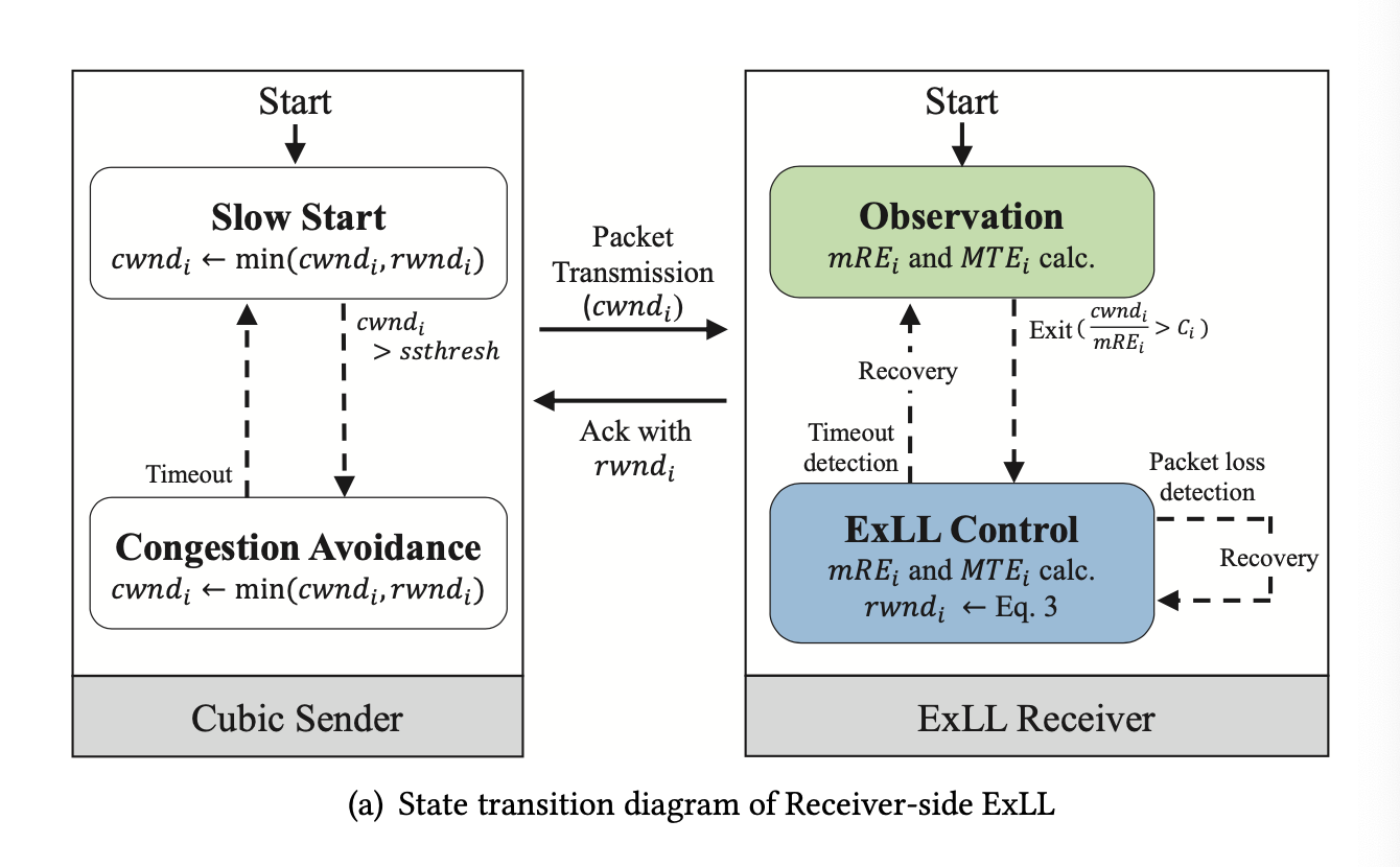
-
Sender-driven: plug-in for Cubic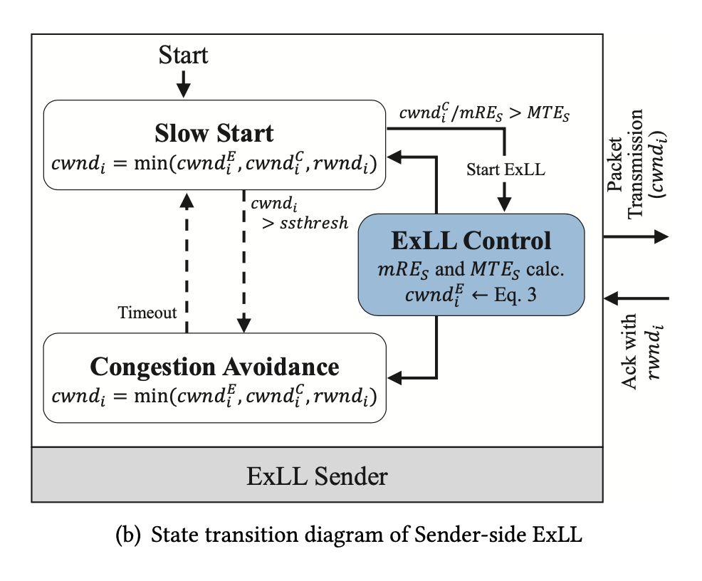
- ExLL Control mode
- When \(\frac{cwnd^C}{mRE_S} > MTE_S\)
- Calculate $ cwnd^E_i $ from Eq.3
- Overrides Cubic when $ cwnd^E < cwnd^C $
-
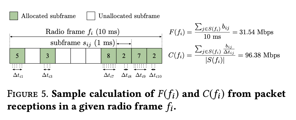
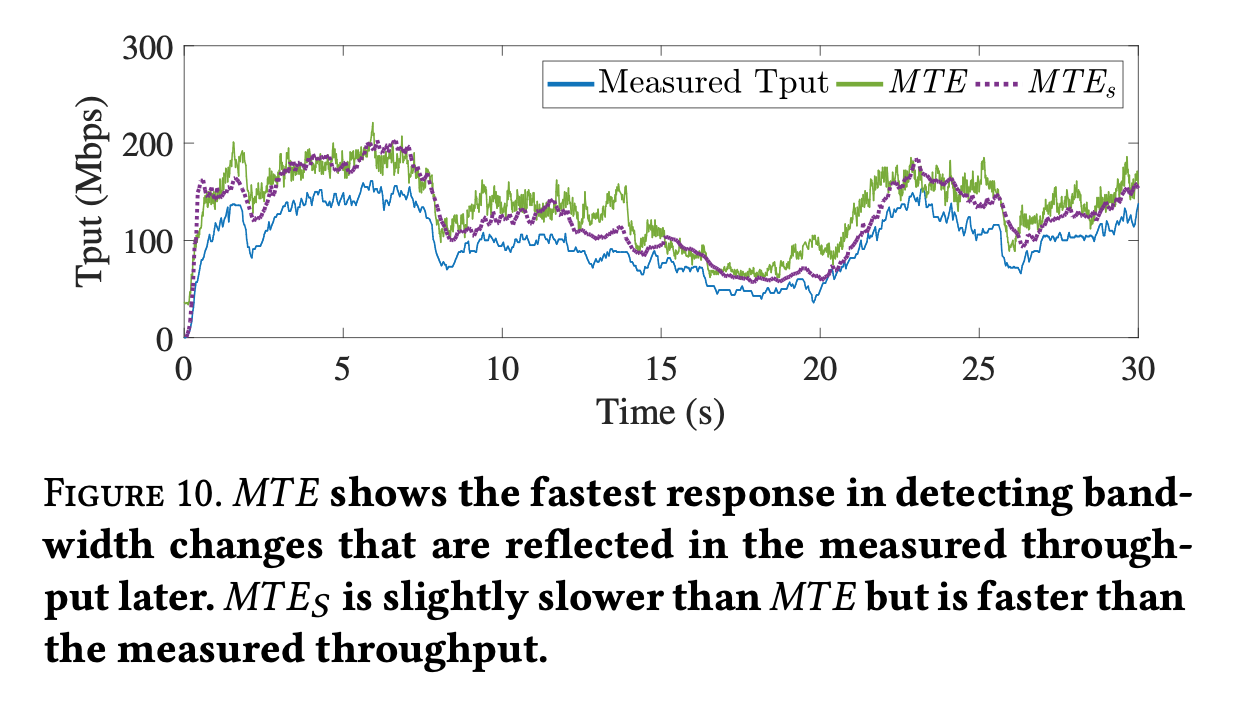
MTE calculation
- F(·) is updated per radio frame = 10ms, much fast than sender’s information delayed by RTT ~ 40+ ms.
- Sender-drive: $ MTE_S = \frac{cwnd}{\Delta t} $ , where $ \Delta t = t_{last Ack} - t_{first Ack} $, small difference in actual experiment measurements
-
mRE calculation
-
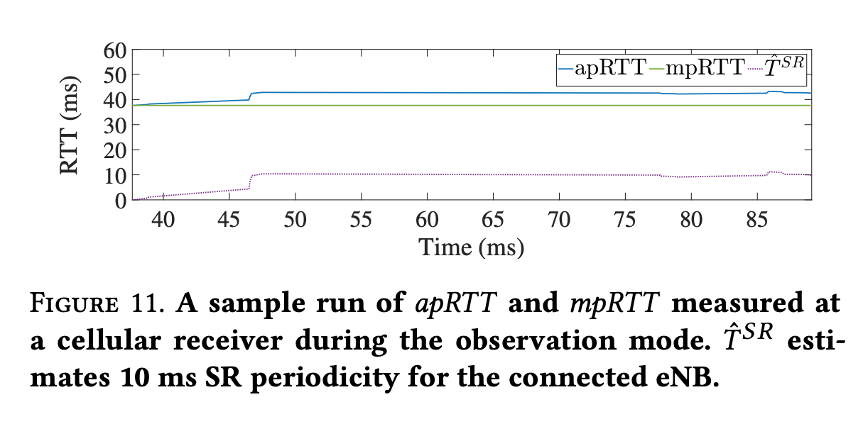
Observation: track minimum, average RTT per packet with mpRTT, apRTT
-
Control
- $ mRE = mpRTT + D(2*(apRTT - mpRTT)) $
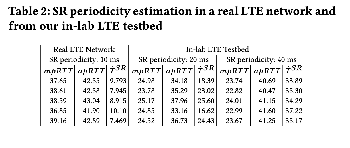
Where D(·) finds matching SR periodicity in (5, 10, 20, 40, 80) from
$ \hat T^{SR} = 2*(apRTT - mpRTT) $
-
Recovery from loss or timeout
- CWND reduced to < RWND for packet loss
- Store RWND value, stop updating RWND until CWND >= RWND again
- Cubic resets, CWND = default initial CWND, for timeout
- Restart ExLL from observation mode
Evaluation
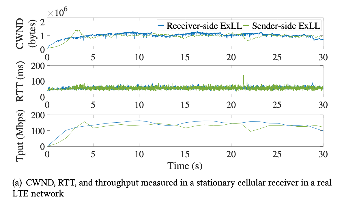
- Receiver- vs. sender-side ExLL: marginal difference, receiver-side slightly better
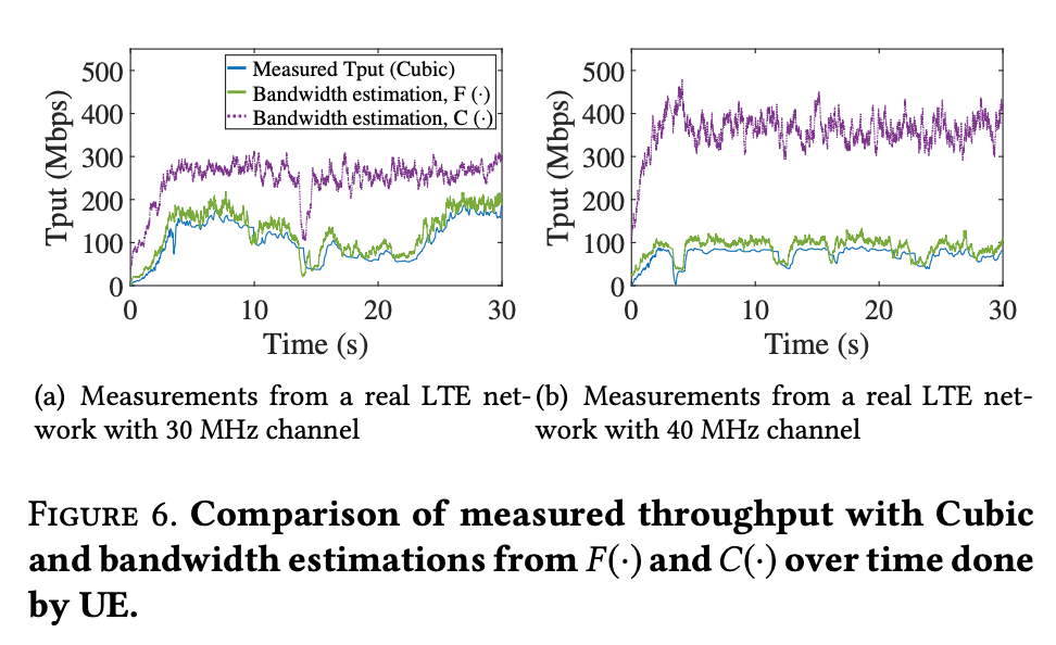
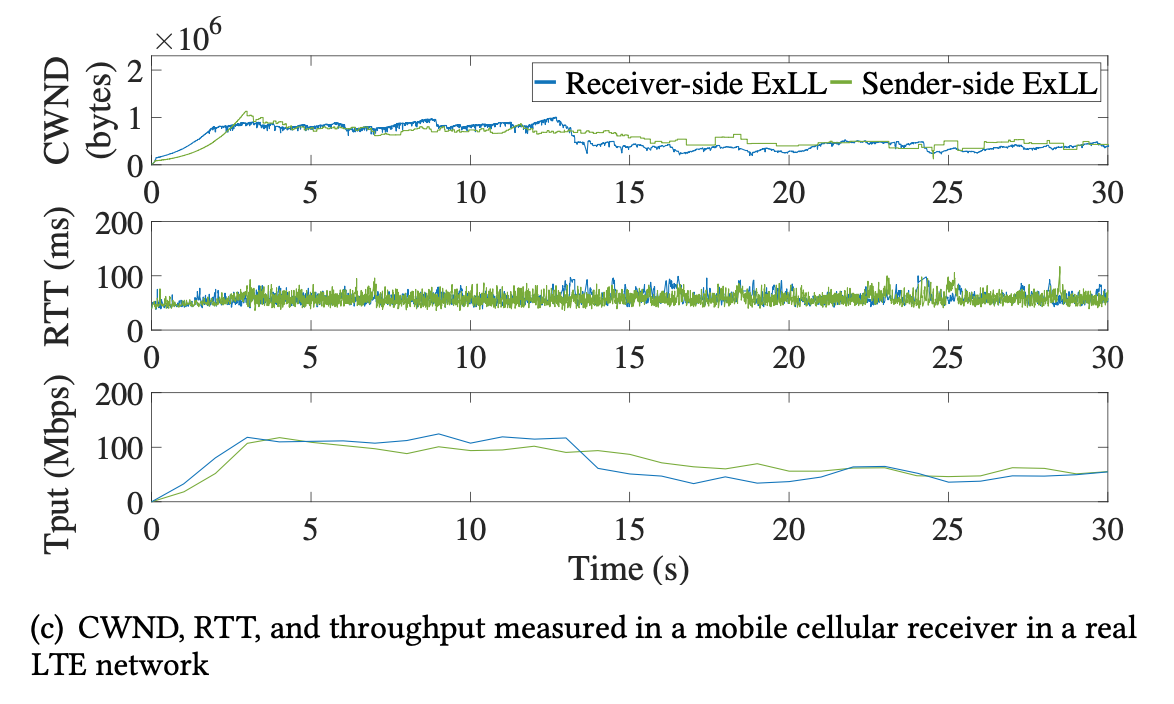
- A real LTE network, mRTT = 50ms, max throughput = 150 Mbps.
- Showing a similar results, stable RTT, throughput, both close to LTE limits.
- CWND of sender-side ExLL less stable.
- In multiple LTE networks
- Sender-side ExLL slightly worse than receiver-side
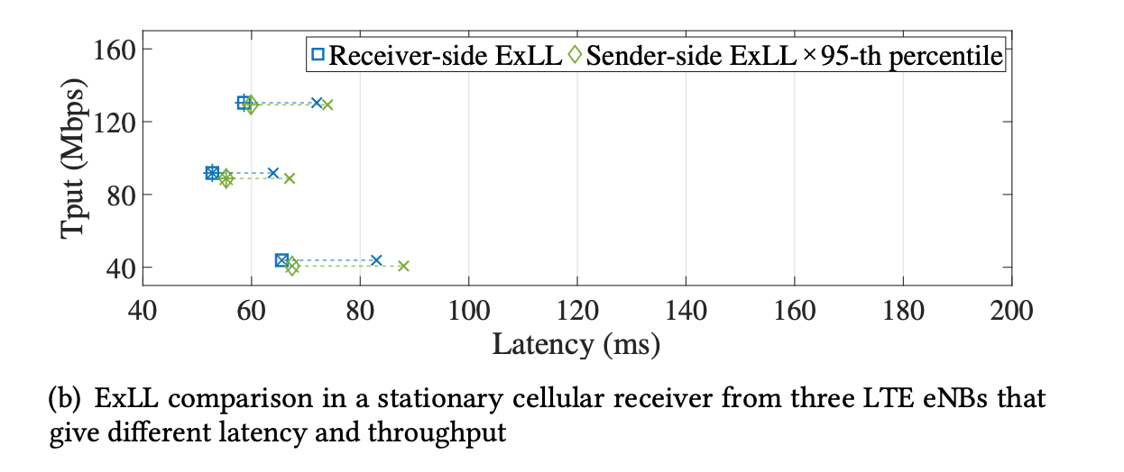
- LTE, RTT = 50ms, Tput = 100 -> 50 Mbps
- Smooth transition from 100 Mbps to 50 Mbps
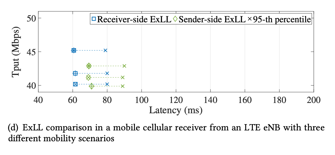
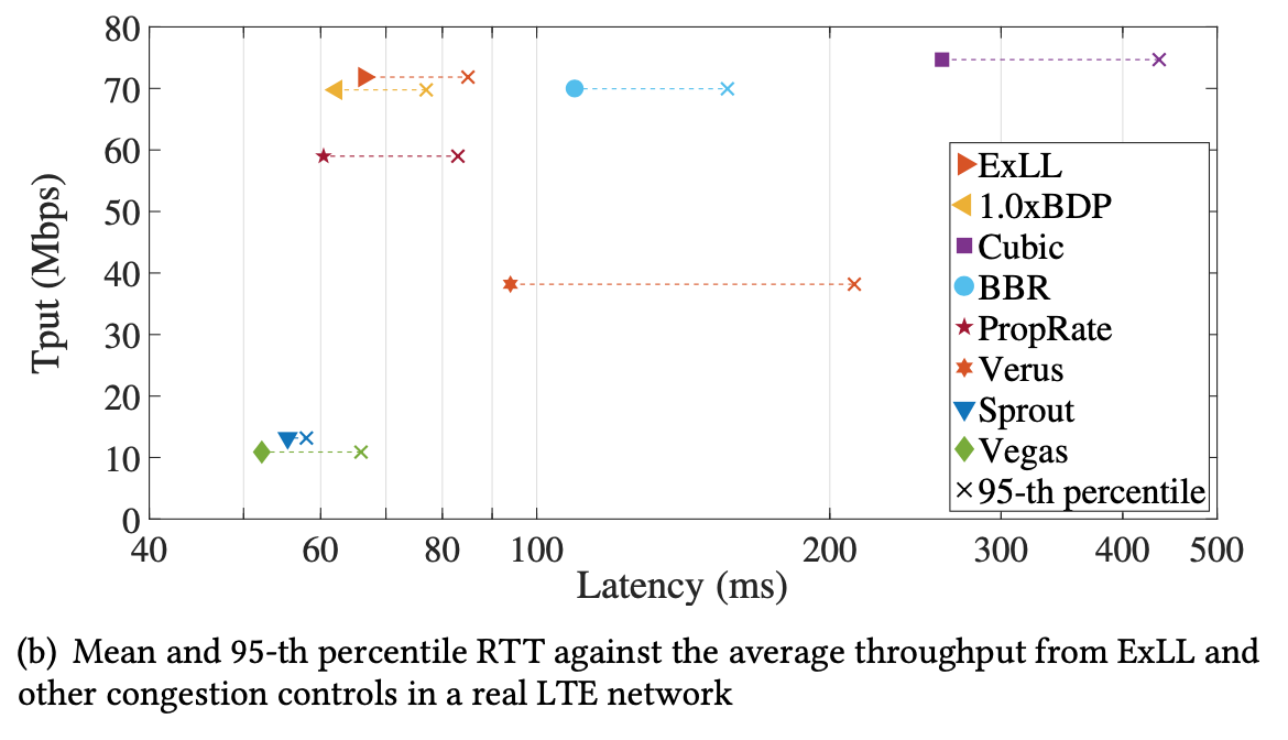
- In different mobility scenarios
- Static Channel:
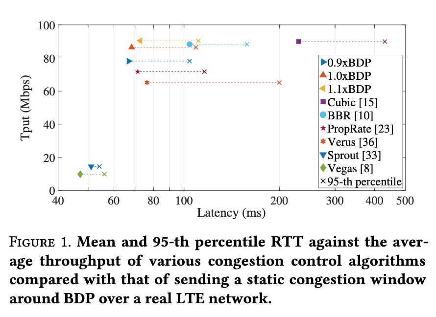
- 90 Mbps, 50ms, ExLL vs. BRR: more accurate RTT, CWND, less fluctuation in throughput
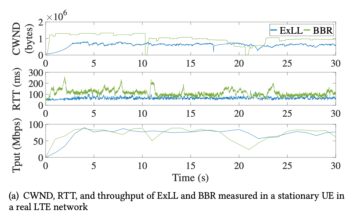
- High throughput, close to Cubic + low latency, close to BDP, PropRate
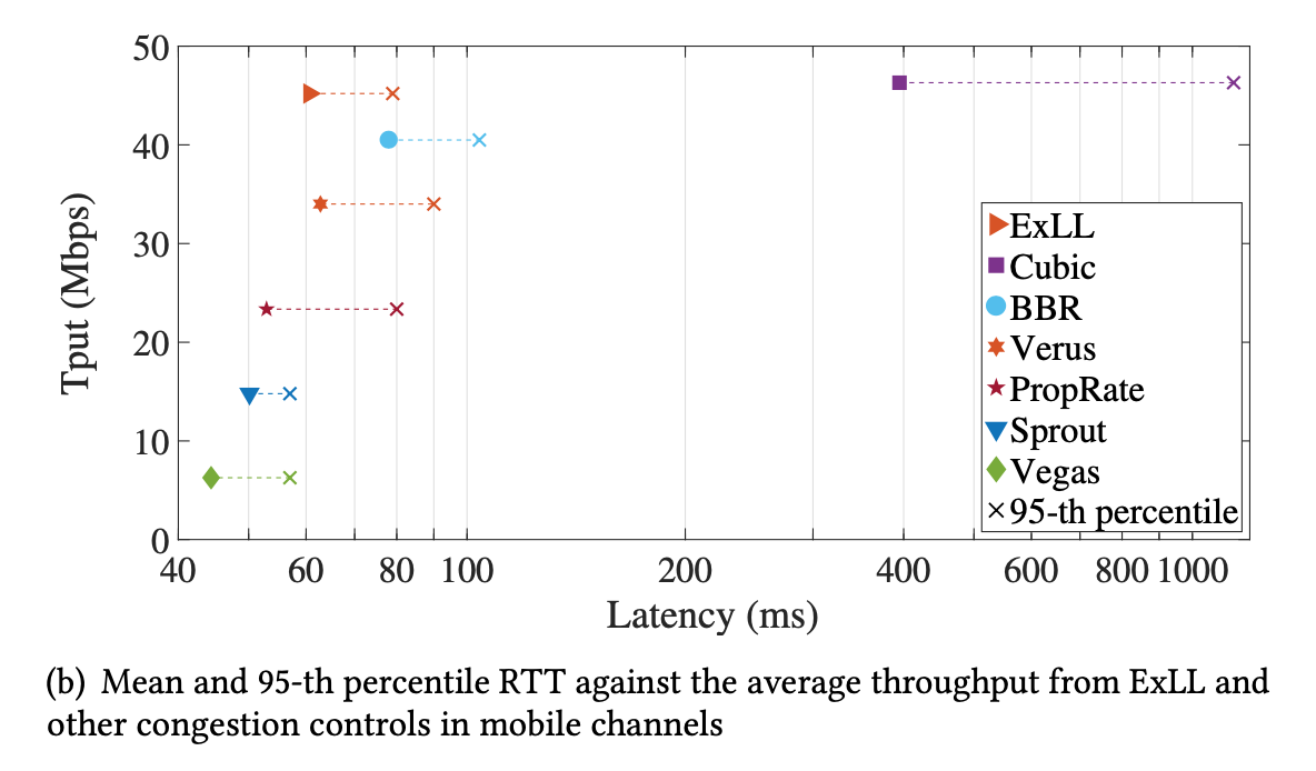
- Mobile Channel
- Smaller RTT, smoother CWND in congested time, 20-40, 80-100
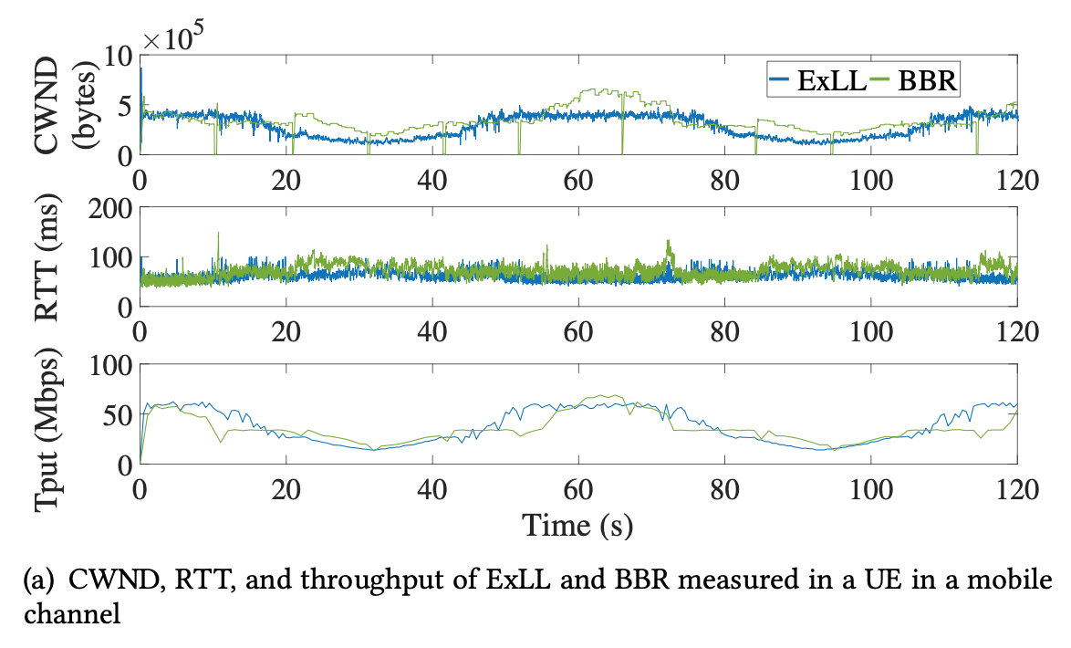
- Outperforms others by a large margin
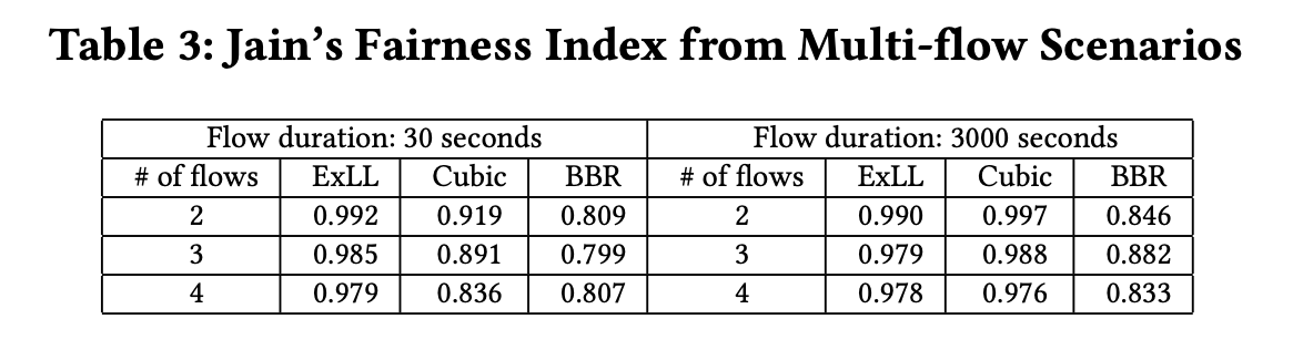
- Multiple Flows
- Fairness (Tput) much better than BRR

- Non-cellular bottleneck adaptation
- 0-30s: non-cellular bottleneck: observation mode
- 30-60s: cellular bottleneck: control mode
- beyond 60s:non-cellular bottleneck: observation mode
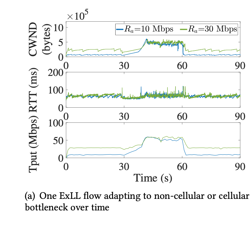
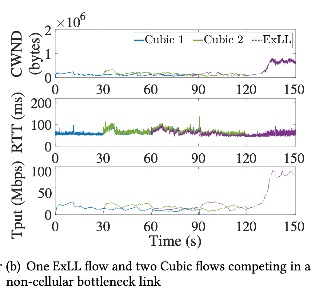
- Runs as Cubic for fairness in first 120s, when non-cellular bottleneck disappears, fully utilize bandwidth
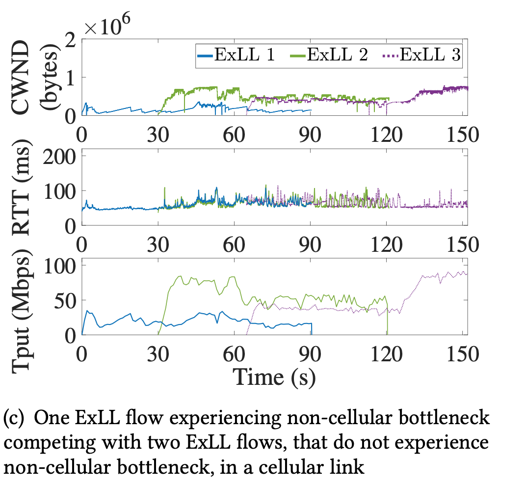
- Fair share of bandwidth with other ExLL flows
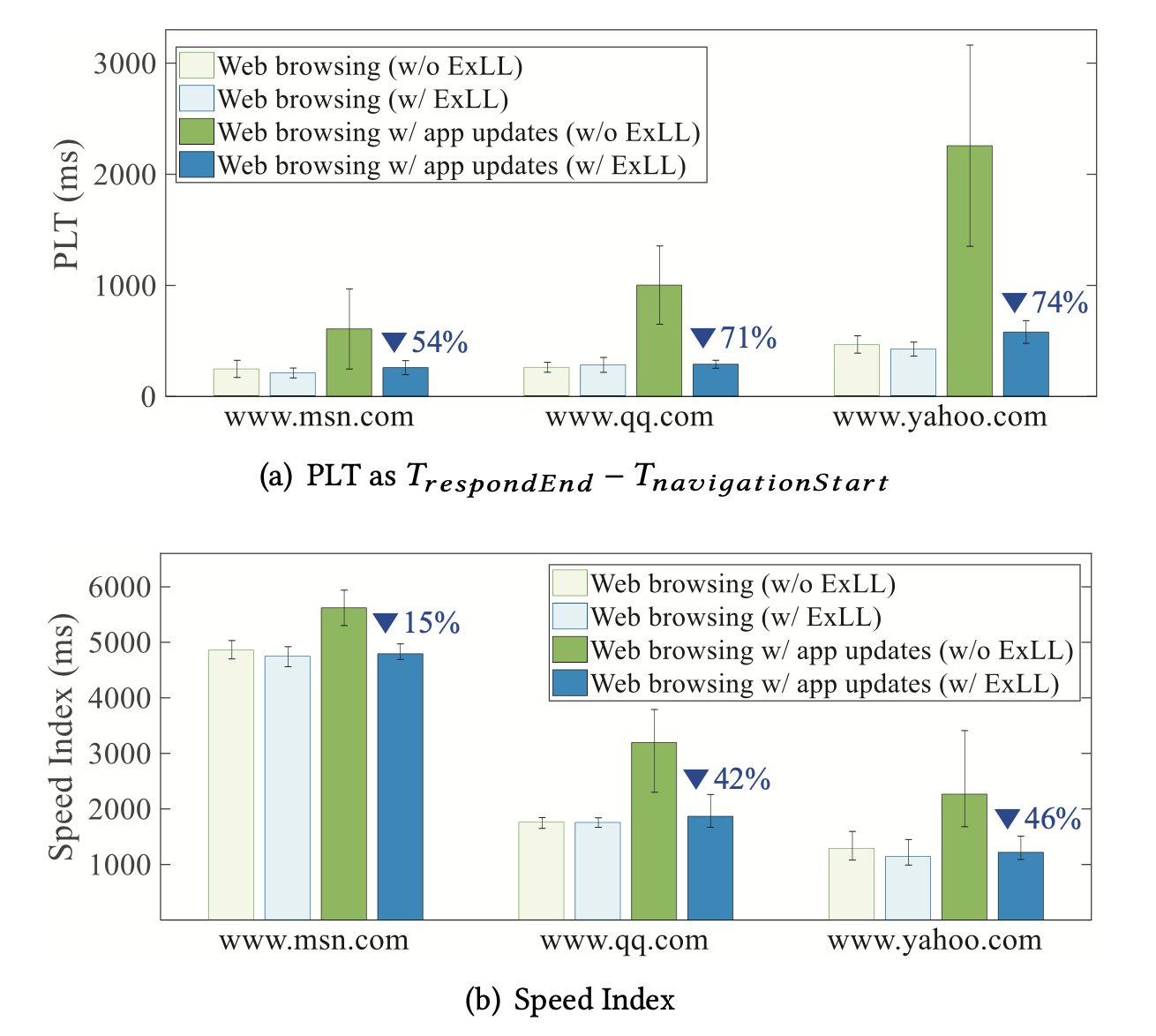
- Showed significant amount of improvement on applications level speed
- For Internet
- Vegas, FAST: Limited deployment, complex.
- BBR: high latency
- Copa: low throughput
- For Datacenter
- pHost: unrealistic assumptions: core is free, size of flows is known in advance
- ExpressPass: new switch function, overhead in packets
- For Cellular:
- DRWA, CQIC, Verus, CLAW, PropRate: worse performances
Conclusion
- Develop novel techniques that can estimate the cellular link bandwidth and realistic minimum RTT without explicit probing, which can be easily extended to next-generation cellular technologies such as 5G.
- Incorporate the control logic of FAST into ExLL to minimize the latency even in dynamic cellular channel conditions.
- Implement ExLL in both receiver- and sender-side versions that give wider deployment opportunities. The receiver-side ExLL can provide an immediate solution for untouched commodity servers while the sender-side ExLL can provide a fundamental solution for 5G URLLC (ultra reliability and low latency communication).
03 Feb 2020
** This is a study & review of the HPCC paper. I’m not an author.
Paper Study: HPCC High Precision Congestion Control
Background
- New trends in datacenter architecture / applications
- Disaggregation datacenter & heterogeneous computing are on the rise: they need low latency and large bandwidth for performance at application level.
- High I/O applications (AI, ML, NVMe) are on the rise: they move large amount of data in a short amount of time. CPU & memory are fast enough –> network is the bottleneck
-
Other attempts failed to reconcile low latency, high bandwidth utility, and high stability because their proposed RDMA architecture can not handle control storms (low utility) and queueing (high latency) properly.
- They believe the existing congestion control algorithm within RDMA is flawed: slow convergence (many guesswork due to coarse-grained feedback signals low bandwidth utility), long packet queueing (long queue when congestion detected, high latency), complicated parameter tuning (more parameters to set up means more chance of human error, low reliability)
HPCC Intro
Experience and Motivation
- Goals
- Latency: as low as possible
- Bandwidth utility: as high as possible
- Congestion & PFC pauses: as few as possible
- Operation complexity: as low as possible
- Trade-off in current RDMA CC, DCQCN: Data Center Quantized Congestion Notification
- Uses ECN (Explicit Congestion Notification) to detect congestion risk by default
- Throughput vs. Stability
- High utilization -> High sensibility & aggressive grow -> easier buffer overflow & oscillation in flow rate –> low stability, vise versa.
- Scheduling Timer
- aggressive timer in favor of throughput vs. forgiving timer in favor of stability.
- Traffic oscillation when link fails
- ECN congestion signaling: low ECN threshold for latency vs. high ECN threshold for bandwidth utility.
-
Metrics for next generation CC
- Fast converge: utility rate quick grows to network limits.
- Close-to-empty queue: short buffer queue
- Few parameters: adapt to environment and traffic itself, less human intervention.
- Fairness: fair distribution among traffic flows.
- Easy hardware deployment: compatible with NIC and switches
-
Commercialization circumstances: INT-enabled hardware and programmable NIC growing in the commercial market
Design
-
HPCC is sender-driven, each packet will be acknowledged by the receiver.
-
Uses INT-enabled switches for fine-grained information on timestamp, queue length, transmitted bytes, and link bandwidth capacity.
-
Idea: limit total inflight bytes in order to avoid congested feedback signal.
-
Sender limits inflight bytes with sending window of W = B * T, where B is NIC bandwidth, T is RTT, plus packet pacer at rate R = W/T.
-
When total inflight bytes is greater than bandwidth, its guaranteed to have congestion, thus to avoid congestion, controlling inflight bytes to be smaller than bandwidth.
-
Estimating inflight bytes by sender: I = qlen + txRate * T, qlen is queue length, txRate is output rate, and txRate = (ack1.txBytes - ack0.txBytes) / (ack1.ts - ack0.ts)
-
Reacting to the signals: Adjust window so that I~j~ is slightly smaller than B~j~ × T, Normalized inflight bytes of link j is :
U~j~ = I~j~ / (B~j~ × T) = (qlen~j~ + txRate~j~ × T) / (Bj × T) = qlen~j~ / (B~j~ × T) + (txRate~j~ / B~j~)
-
Sender i react to the most congested link:
W~i~ = W~i~ / max~j~ × k~j~ + W~AI~
- Idea: use RTT + ACK reaction to overcome trade-off between quick reaction vs. overreaction
-
Workflow
- New ACK message triggers NewAck() function
- When ACK sequence number is new, updates window size, also recalculates INT info
- Function MeasureInflight estimates normalized inflight bytes with Eqn (2) at Line 5
- Function ComputeWind combines multiplicative increase/ decrease (MI/MD) and additive increase (AI) to balance the reaction speed and fairness.
-
Parameters
- η: bandwidth utility rate, default to 95%
- maxStage: stability vs. speed of reclaim free bandwidth, default to 5
- W~AI~: max number of concurrent flows + speed of converge vs. fairness
- Advantages of HPCC vs others
- Prototyped with NIC with FPGA programmability + switching ASICs with P4 programmability. Compared to DCQCN on the same platform.
Evaluation
- Faster & better flow rate recovery: pic 9a, 9b
- Faster & better congestion avoidance: pic 9c, 9d
- Lower network latency: pic 9e, 9f
- Fairness: 9g and 9h
- Significantly reduces FCT for short flows: pic 10a, 10c
- Steadily close-to-zero queues: pic 10b, 10d
- Good for short flows as HPCC keeps near-zero queues and resolves congestion quickly: pic 11a, 11b, 11c, 11d
- Good for long flows as HPCC allows 5% bandwidth headroom, long flow has a higher slow-down: pic 11a, 11c
- Good for stability as HPCC reduces PFC pauses to almost zero: pic 11b
- RDMA CC:
- TIMELY: incast congestion, long queues.
- iWarp: high latency, vulnerability to incast, high cost.
- General CC for data center networks:
- DCTCP & TCP Bolt: high CPU overhead, high latency, long queue
- Proposals to reduce latency
- qFabric: complex logics in switches
- HULL: allocate bandwidth headroom, similar to HPCC, but requires non-trivial implementations on switches for Phantom queues to get feedback before link saturation.
- DeTail: needs new switch architecture
- HOMA & NDP: receiver-driven, credit-based solution
- Flow controls for RDMA: to reduce hardware-based selective packet retransmission to prevent PFC pauses or to replace FPC
- IRN & MELO: complementary with HPCC, worse results than HPCC
04 Jan 2020
Computer System Architecture Labs
The lab is a simulation of a pipelined MIPS processor with C++ as part of my school project. The code simulates basic pipelined processor components including Memory, Registers and ALU. It supports dependency-resolving techniques such as stalling, forwarding. This simulation is five-staged: Instruction Fetching (IF), Instructions Decode (ID), Execution (EX), Memory (MEM), Write Back (WB).
Code and project specification can be found here.
01 Oct 2019
An Introduction to My Word2Vec Application
At China Media Cloud, I’ve worked on multiple applications involving Word2Vec models. The basic idea behind Word2Vec is to represent words with vectors in order to use mathematical properties of vectors to perform calculations with words. The majority of my work on Word2Vec models is done with Python’s CoreNLP, developed by Stanford University, and Gensim, an awesome package for Word2Vec modeling. Both are open source.
Some of the things I did was:
- Identify customer business need that can be fulfilled with Word2Vec models.
- Collect training data with internal APIs and database.
- Preprocess, format, and label data for training.
- Use Gensim to train Word2Vec models.
- Incorporate Word2Vec models into Smart Editor web application.
Before any programming, I was asked to research common NLP models, packages, and their applications with a senior engineer. We had meetings with product managers, clients, and tech VP of the company to discuss how we can incorporate NLP technologies into out existing products for more functionalities and services. After settling down to a few packages, namely CoreNLP for Entity Recognition, Part-Of-Speech Identification, and Gensim for Word2Vec, I started to work on the training data.
If there’s one thing I’ve learned from the projects, that is the training data is utterly important in any machine learning/deep learning tasks. I spent a major chunk of my time working on the cleaning (getting rid of the scrambled words and characters), parsing (easy for english, but can be very tricky for non-space-separated languages, such as Chinese or Japanese), and formatting (often involving some yield function to reduce memory use) the textual data in order to make the training easier.
To put it very simple, a Word2Vec model is a neutral network that translates words into vectors. A simple, but not that simple, introduction to Word2Vec can be found here. Word2Vec is a great idea in terms of computability because computers can work with vectors and numbers much more easily and effectively than strings of characters. My work involves training multiple Word2Vec models with the training data I prepared in advance, and utilize the models for higher-level tasks.
Because the fact that the model generates a spacial distribution of the words during training, it can compute the synonym or antonym with some simple matrix computation. While the model technically can’t understand the semantic meanings, it can find relationships of a word to other words. With this technique, we’ve built a relevance-reveal system where the user will get a radar map of relative words with relevance level for his/her selection. Several models were trained for different news categories to improve their accuracies. For example, an ESPN sports editor wants to write about basketball. He selects the word “Los Angeles Lakers” for a search, and the sports news Word2Vec model (trained with sports news) will return a list of relative keywords such as “LeBron”, “Kobe”, or “Rockets” and their associated relevance level to help the editor to expand his writing. The models were loaded in the server, and updated from time to time with newly collect news data. I also wrote RESTful APIs for this function and added a censor mechanism to filter return values per client requests.
Another application of the Word2Vec models is the News Classifier that I worked on. The Word2Vec model acts as the embedding layer (which transform string of characters into vectors) of the News Classifier CNN and works very well because it was trained with the news data that were to be classified by the classifier and adjusted accordingly. I will write more about the News Classifier later.
Last Modified: 10-15-2019