28 Apr 2020
** This is a study & review of the Opera paper. I’m not an author.
A New Adaptive FEC Loss Control Algorithm for Voice Over IP Applications
Introduction
- Problem with previous schemes: can’t handle burst loss and show unstable behaviors
- Section 2: application-level packet-loss techniques Bolot’s algorithm
- Section 3: Shortcomings of Bolot’s algorithm
- Section 4: New Design USF algorithm
- Section 5: Simulation
Application-level packet-loss recovery & Bolot’s algorithm
Pre-specified HIGH and LOW limits for loss rate. Add redundancy when the loss rate is higher than HIGH, and decrease redundancy when the loss rate is lower than LOW.
Redundancy level depends on Combination Number:
Reward measures the audio quality at the receiver (loss rate before vs after reconstruction) (empirically determined)
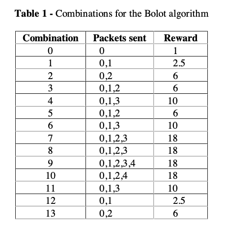
A RTCP packet contains the number of packets lost before reconstruction at receiver in the last 5s.
For each RTCP received:
	# Packet Loss Rate Before Reconstruction
	Pb = lost packets / total packets expected
	# Packet Loss Rate After Reconstruction
	Pa = Pb / Reward
	if Pa > HIGH: # Loss after reconstruction still too large (network congested)
		combination++
	if Pb < LOW: # Loss before reconstruction small enough (good network condition)
		combination--
Shortcomings of Bolot’s Algorithm
Static and empirically determined reward number $\rightarrow$ representative for a limited scenarios (only for those similar to the testing condition)
Bolot’s algorithm doesn’t consider change in packet loss rate before reconstruction $\rightarrow$ with poorly set HIGH and LOW value $\rightarrow$ fluctuation. For example, if we set both HIGH and LOW at 3%, then one RTCP increases redundancy and the other reduces redundancy, forming a cycle of fluctuation.
New AFEC: USF algorithm
Add two additional values in the RTCP packets.
- The number of packets lost after reconstruction, used to calculate the actual percentage of packets loss after reconstruction.
- Total number of packets lost in bursts, used to account for burst loss.
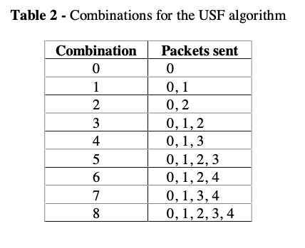
USF first increases delay and then add more redundancy to the traffic.
For each RTCP:
	# Packet loss rate after reconstruction
	Pa = Number of Packets lost after reconstruction / Total number expected
	# Packet loss rate before reconstruction
	Pb = Number of packets lost before reconstruction / Total number expceted
	if Pa > HIGH: # calebrate for burst loss
		subtract burst loss from loss
		recalculate Pa with the new loss
        if Pa > HIGH: # lost still high
            increment combination
	if Pa < LOW: # low loss rate
		loss difference = Pb(previous) - Pb
        if loss difference > threshold:
            decrement combination
	Pb(previous) = Pb
Main point: safe guard increment and decrement from burst loss and fluctuation.
Simulation and Evaluation
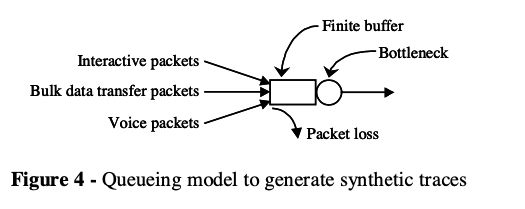
VoIP stream at period of 20 ms. Each packet is numbered for loss tracking.
Used Interactive (telnet), Bulk Data (FTP) to simulate realistic traffic, adjust for different VoIP loss rate.
- With relatively stable and good network (loss around 3%)
HIGH and LOW @ 3%. USF threshold @ 3%. (3% loss rate for a tolerable audio quality)
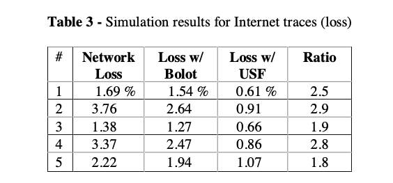
Table 3: USF reduces loss rate at 2-3X.
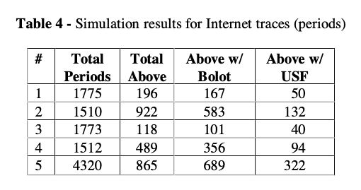
Table 4: Period of 5s (RTCP); number of these periods above HIGH.
Fewer above HIGH periods means that USF can effectively handle high loss (when network condition becomes bad) by increasing redundancy level.
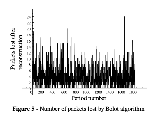
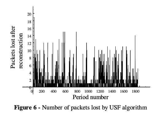
Compare figure 5 against 6, we can see the number of packet loss after reconstruction with USF is significantly less.
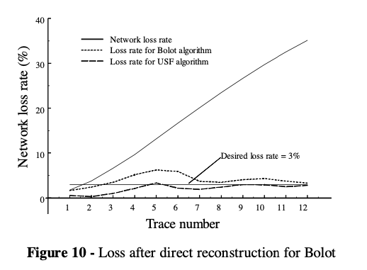
- Synthetic network (network loss rate varies from 2%-35%)
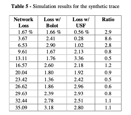
For network loss < 7%, USF performs well. But when network is heavily congested and loss rate is high, USF struggles. Confirms in figure 8.
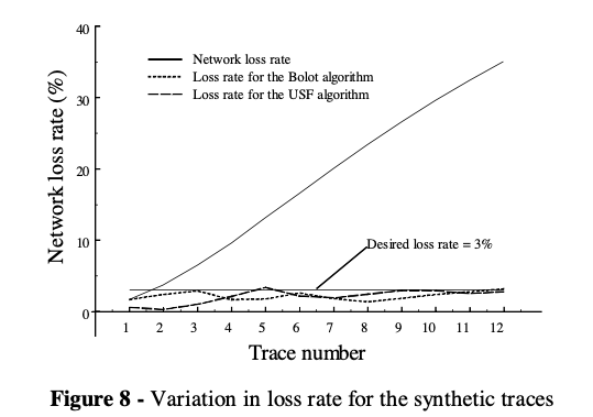
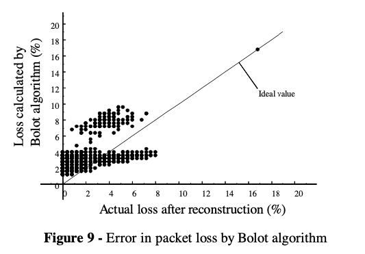
Why would Bolot outperforms USF with higher network loss? Bolot often overestimates loss rate after reconstruction (Figure 9: dots concentrates above the actual loss rate after reconstruction line) $\rightarrow$ over-redundant $\rightarrow$ performs well in bad network conditions
What if Bolot also uses actual loss rate after reconstruction like USF? USF outperforms Bolot for all range.
Conclusion USF AFEC
- Clearly USF AFEC is good when the network condition is relatively stable and well, but struggles otherwise
- It uses actual network loss to compute redundancy $\rightarrow$ more accurate measure of AFEC effectiveness.
- It calibrates for burst loss and consider network loss history when making redundancy changes $\rightarrow$ less frequent change $\rightarrow$ less fluctuation
- Needs more works on LOW, HIGH, threshold setting? Bandwidth Util? Improve for high loss rate conditions?
10 Mar 2020
** This is a study & review of the Opera paper. I’m not an author.
ABC
Intro
- A new explicit congestion control protocol for network paths with wireless links
- Existing explicit control protocols (XCP, RCP, specify a target rate for sender and receiver) problem
- designed for fixed-capacity links, no good performance in wireless network
- require major changes to packet header, router, endpoints to deploy
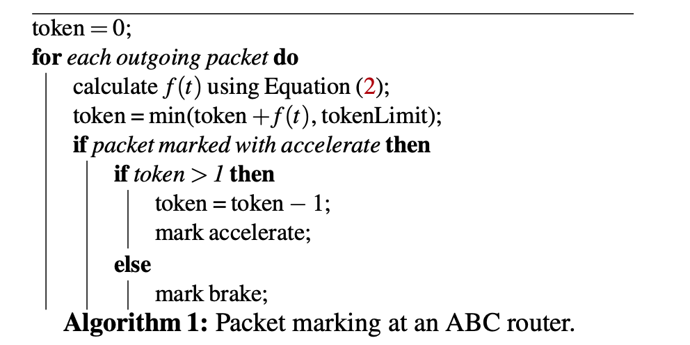
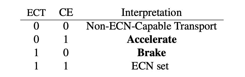
- Simple mechanism: a wireless router marks each packet with either accelerate or brake with two bits, sender receives this marked ACK to enlarge and shrink sending window size
- Accurate feedback & measurement for link condition
- XCP, RCP compares enqueue rate with link capacity
- ABC router compares dequeue rate with link capacity, because dequeue rate is a more accurate indication of how many packets will be arriving in next RTT
- Can be deployed on existing explicit congestion notification (ECN) infrastructure
Motivation
-
Main challenge: wireless link rates vary largely and rapidly, hard to achieve high throughput and low delay
-
End-to-end congestion control
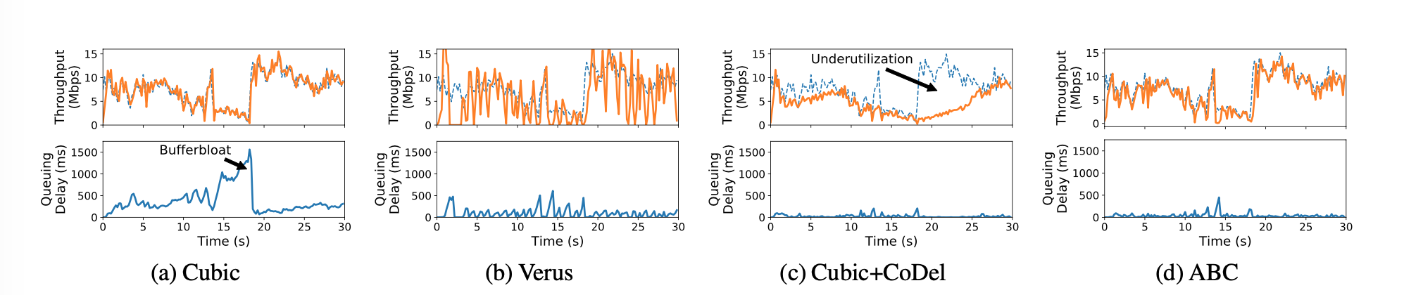
- Cubic (a)
- Rely on packets drop to infer congestion.
- Large buffer, long queue, large delay
- BBR
- Uses RTT and send\receive rate to infer congestion condition
- can cause underutilization
- Verus, Sprout (b)
- Uses a parameter to balance aggressive(large queue) and conservative(low utilization), tradeoff
-
Active Queue Management (AQM) schemes
- RED, PIE and CoDel (c)
- signals congestion, but do not signal good link condition
- underutilization
-
Deployment
- XCP, RCP requires modification of header, router, endpoints. Not very compatible with existing infrastructures, some router drops packets with IP options, TCP options is problematic for middle-box (firewall, etc) or IPSec
- Fairness to older routers
-
Goals
- Control algorithm for fast-varying wireless links
- No modifications to packet headers
- Coexistence with legacy bottleneck routers
- Coexistence with legacy transport protocols
Design
-
ABC senders receives an
- accelerate ACK, increases congestion window by 1, effectively sending 2 packets, 1 for ACK & 1 for window size increase
- brake ACK, decreases congestion window by 1, effectively stops sending packets in response to the decrease in congestion window size
-
effectively this scheme can double (all accelerate ACK) or zero (all brake ACK) the current congestion window in one RTT
-
Target rate is calculated with $tr(t)=\eta\mu(t)-\frac{\mu(t)}{\delta}(x(t)-d_t)^+$, where $μ(t)$ is the link capacity, $x(t)$ is the observed queuing delay, $d_t$ is a pre-configured delay threshold, $η$ is a constant less than 1, $δ$ is a positive constant (in units of time), and $y^+$ is $max(y,0)$.
if x(t) < dt: 		## queueing delay is low
	target = ημ(t)  ## η = 0.95, slightly below bandwidth for delay reduction
else: 				## queueing delay is higher than threshold
	target = ημ(t)-(μ(t)/δ)(x(t)-dt) ## reduce the amount that causes the queueing delay to decrease to dt in δ seconds
-
Marking (how much should be marked accelerate) fraction is calculated with $f(t)=min(\frac{tr(t)}{2cr(t)}, 1)$, where $cr(t)$ is the dequeue rate.
-
enqueue rate vs dequeue rate:
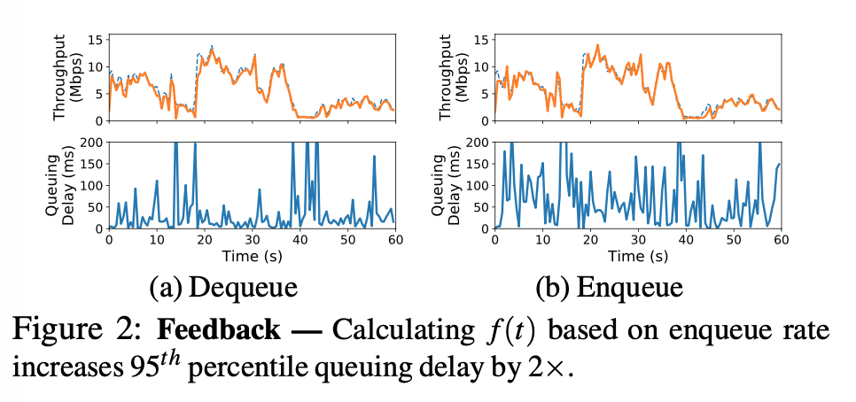
- $f(t)$ is calculated with every outgoing ACK, thus granting quicker adjustments to the network condition than periodical schemes (XCP, RCP) with the following algorithm to ensure no more than a fraction of $f(t) $ of packets are accelerate ACKs.
- Fairness is achieved with the following algorithm $w\leftarrow \begin{cases}
w+1+1/w \text{ , if accelerate}
w-1+1/w \text{ , if brake}
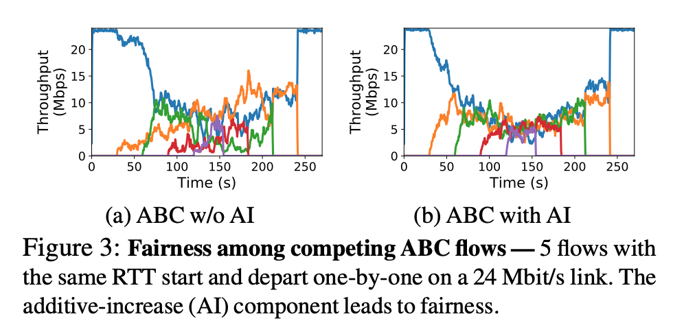
\end{cases}$ , which includes additive increase (AI), but still suffer from RTT unfairness: the throughput of a flow is inversely proportional to its RTT, like Cubic.
Deployment
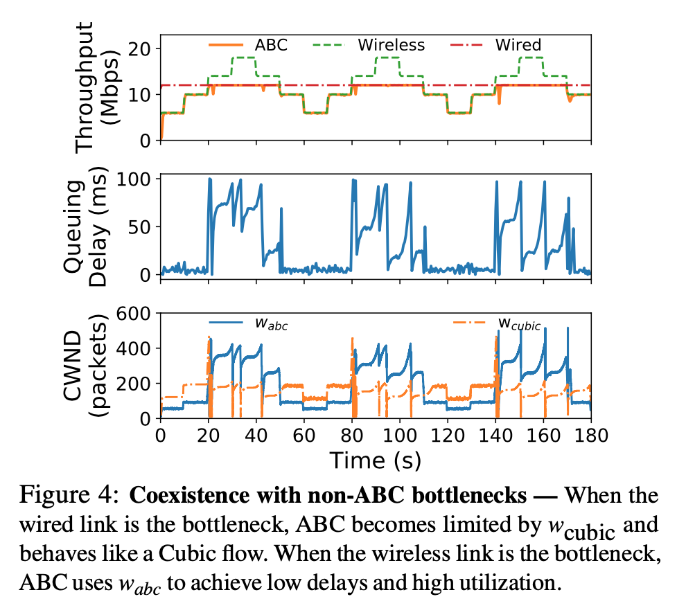
- coexistence with non-ABC routers: must be able to react to traditional congestion signals (drops or ECN) $\rightarrow$ keeping two link rates, one for ABC rate, not for non-ABC rates, use smaller one
- problem: when non-ABC router is bottleneck $\rightarrow$ ABC rate continuously grow
- solution: caps both ABC rate and non-ABC rate at 2X # of packets in-flight
- Protocol implemented with ECN bits
- legacy ECN bits
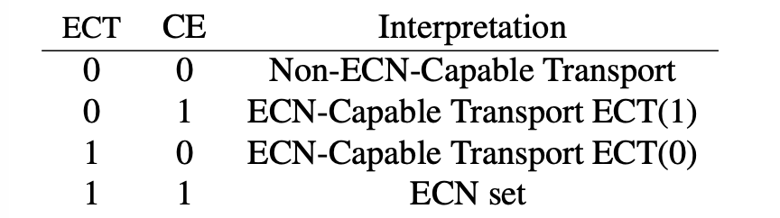
- ABC bits
- Only needs to modify receiver software
Discussion
- Delayed ACK: uses byte counting at the sender, sender in/decreases its windows by the new bytes ACKed, keeps track of state (acc/brake), once state changes, sends a ACK for state change
- Lost ACK: ABC can handle lost ACK
- ABC routers do not change incoming ECN marks: because ECN does not convey ABC accelerate/brake information, ECN will slow down adjustment. When ECN is small in fraction, adjustment loss is small. When ECN is large in fraction, non-ABC router becomes bottleneck and sender will not use ABC window and rates.
- ECN routers can overwrite ABC acc/brake bits, but will not be a big problem as previous entry suggests
Eval
- On Verizon cellular network, ABC outperforms other protocols
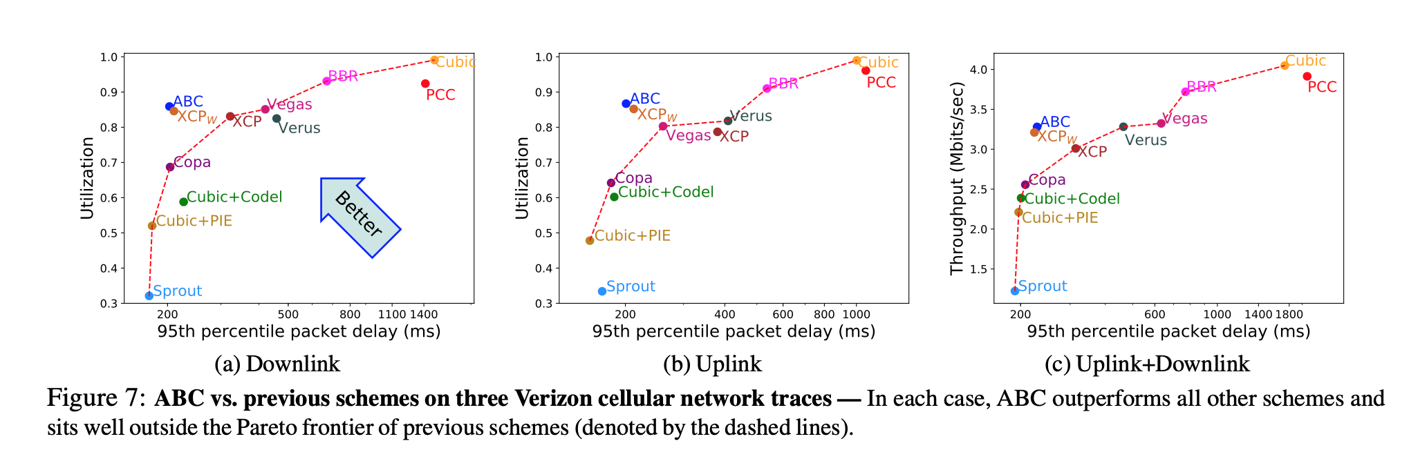
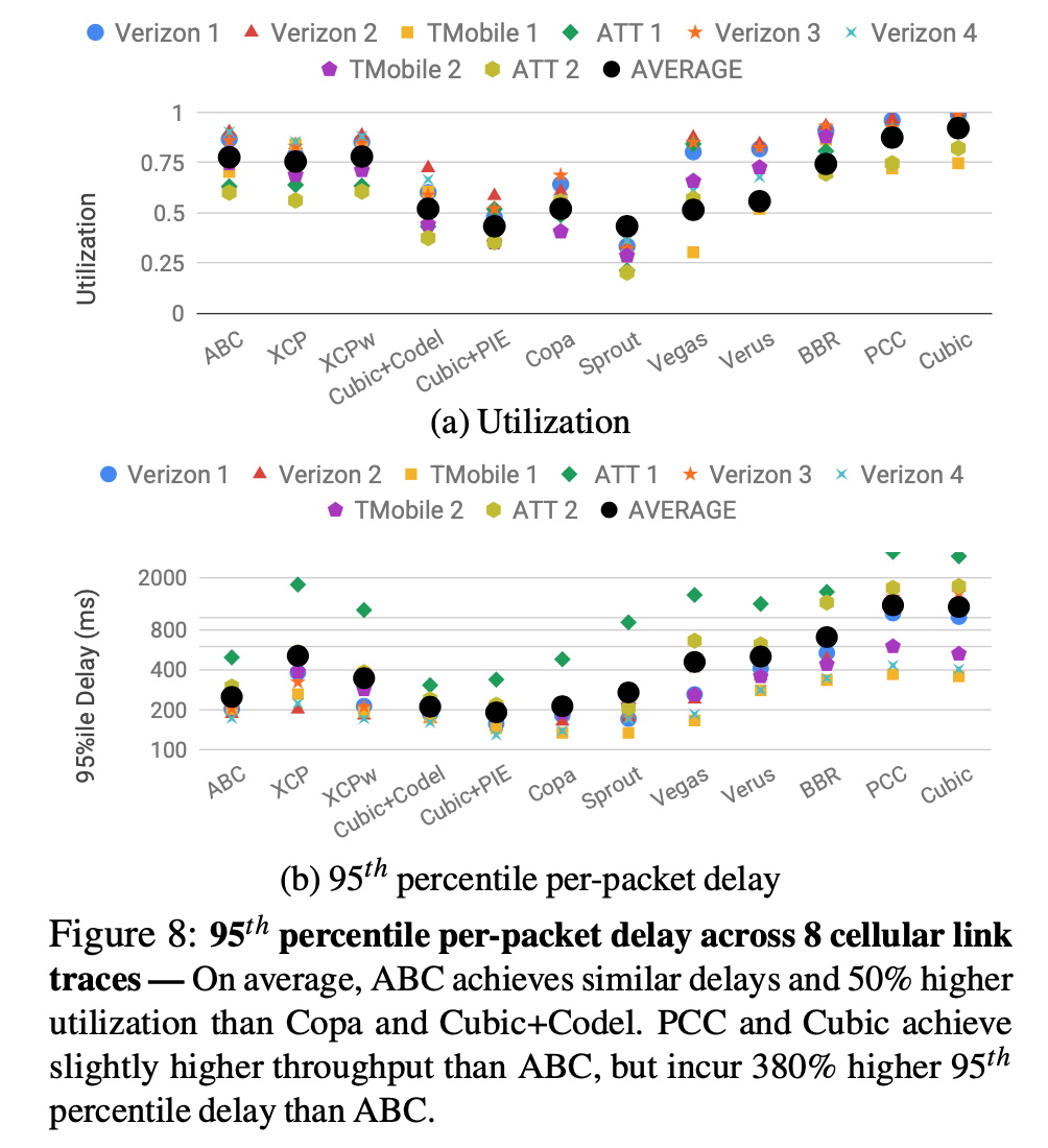
- Tested on 8 different cellular networks against other explicit congestion control scheme: PCC/Cubic achieves higher utilization, but they are considerably higher in delays
- Performance over WiFi with different delay threshold
- black doted line is ideal rate, closely matched with orange line (ABC), low delay when no cross traffic, matches wireless in yellow region (wireless is bottleneck), and ideal in gray region (wired is bottleneck)
- ABC suffers from RTT unfairness, similarly to Cubic
Conclusion
A new explicit (accelerate/brake) congestion control protocol for network paths with wireless links, which is deployable.
a. target rate
target rate is enqueueing rate in 1 RTT
at $T_{RTT=0}$, dequeueing rate $cr(t)$, $f(t)$ of accelerates will comes back with $2*f(t)$ packets in the next RTT
at $T_{RTT=1}$, $tr(t) = cr(t)2f(t)\rightarrow f(t)=\frac{tr(t)}{2*cr(t)}$
For example, when we want steady state; $tr(t)=cr(t)$:
$tr(t)=cr(t)2f(t) \rightarrow f(t)=\frac{tr(t)}{2*cr(t)}=\frac{1}{2}$
$f(t) = 1/2$ to maintain current rate
**b. why not steady state ** percentage change
Because
- wireless link conditions change by a largely and quickly, very unsteady by nature.
- they want to have quick adjustment to the rate, where schemes like DCTCP still is periodical (by grouping ACKs together for analysis), which is slow in adjustment in their opinion
c. link estimation
Who does the job? 802.11n access point (AP) router
Two cases: single user, multiple users
Link rate is defined as the “potential throughput” of the user (e.g. MAC of a WiFi client)
possible solutions
-
use physical layer bit rate (depends on modulation and channel code), but will overestimate link rate (does not count delay for additional tasks, e.g. channel contention, retransmission…)
-
use fraction of time that the router queue was backlogged $\rightarrow$ link underutilization, but WiFi MAC packet batching is problematic for this approach. Batch builds up while waiting for ACK for last batch, but does not indicates that the link is fully utilized
Batching
In 802.11n, data frame (MPDUs) is transmitted in batches (A-MPDUs).
Current Dequeue Rate can be estimated by
\(cr(t)=\frac{b*S}{T_{IA}(b,t)}\)
where $b$ is a smaller batch size $b<M$ (router might send a b-sized batch when not having enough data to send a M-sized full batch ), $M$ is full-sized batch size, frame size S bits, $T_{IA}(b,t)$ is ACK inter-arrival time (time between receptions of two consecutive block ACKs)
When user is backlogged, $b=M$, the estimation equals link capacity.
When user is not backlogged, $b<M$, calculate $T_{IA}(M,t)$, as if the user is backlogged and had sent M frames.
Thus Link Capacity can be estimated by
\(\hat{\mu}(t)=\frac{M*S}{\hat{T}_{IA}(M,t)}\)
Now the problem becomes estimating ACKs interval time $T_{IA}(M,t)$.
ACK interval time = batch transmission time + “overhead” time (e.g. physically receiving ACK, contending for shared channel, transmitting physical layer preamble…) $\rightarrow$
\(T_{IA}(b,t)=\frac{b*S}{R}+h(t)\)
where $h(t)$ is overhead time, R is bitrate for transmission
- for same batch size, interval vary due to overhead
- slope of the line is $S/R$
Thus the ACK Interval Time can be estimated by
\(\begin{align*}
\hat{T}_{IA}(M,t) & = \frac{M*S}{R}+h(t) \\
& = {T}_{IA}(b,t) + \frac{(M-b)*S}{R}
\end{align*}\)
Calculation on every batch transmission, pass through a weighted moving average filter over time T to smooth out. They used T=40ms.
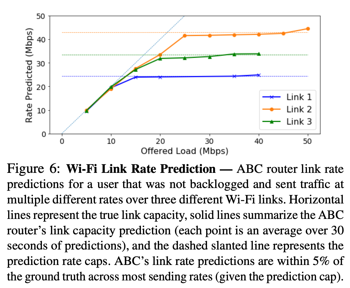
horizontal dashed line: true link capacity
solid line: ABC prediction, very close to true capacity
dashed slope line: ??
Multiple users**
Different users have their own batch size M and transmission rate.
Two scenarios:
Each user calculates a separate link rate estimate. Notable: 1. ACK interval time is on a per-user basis; Overhead time $h(t)$ now includes time when other users are scheduled to send packets. Fairness is ensured.
Router calculates single aggregate link rate estimate. Notable: inter-ACK time for all user ACKs, regardless of which user this ACK belongs to. Use aggregate link rate to guide target rate, and control accelerate-brake ratio. (Fairness not ensured?)
Cellular Networks
Each user has its own queue and link rate. 3GPP provides how to use scheduling information to calculate link rate.
d. why using only two states
No room in TCP header, can’t use IP/TCP options $\rightarrow$ repurpose ECN bits and ECN bits can only be repurposed into two states. Two states are sufficient to handle the adjustment when the number of packets are large enough, because one accelerate will cancel out one brake, thus achieving steady state is not hard.
10 Mar 2020
** This is a study & review of the Opera paper. I’m not an author.
CONTRA
Motivation
In order to achieve efficient routing protocols, a system should supports:
- Traffic Engineering: prefer least utilized paths
- Routing Constraints: middle-box traversal, specifying certain routes
- Fast Adaption: update routing upon condition change
Conga/Hula: supports only least utilized path policy, not RC and not for arbitrary topology (only uses tree-like topo)
Contra: performance aware, programmable, general (for wide range of policies and topologies)
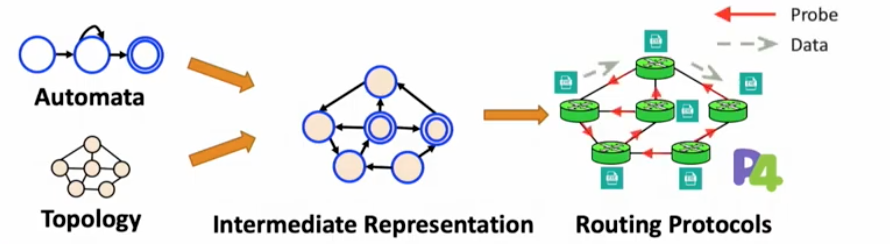
High level view:
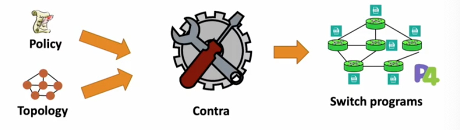
Contra compiles high level policies into performance-aware routing protocols in data plane
Language
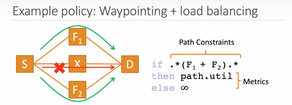
Path constraints are defined with regular expression, metric
Example: S can use F1/F2 with least util to reach D, drop for other path
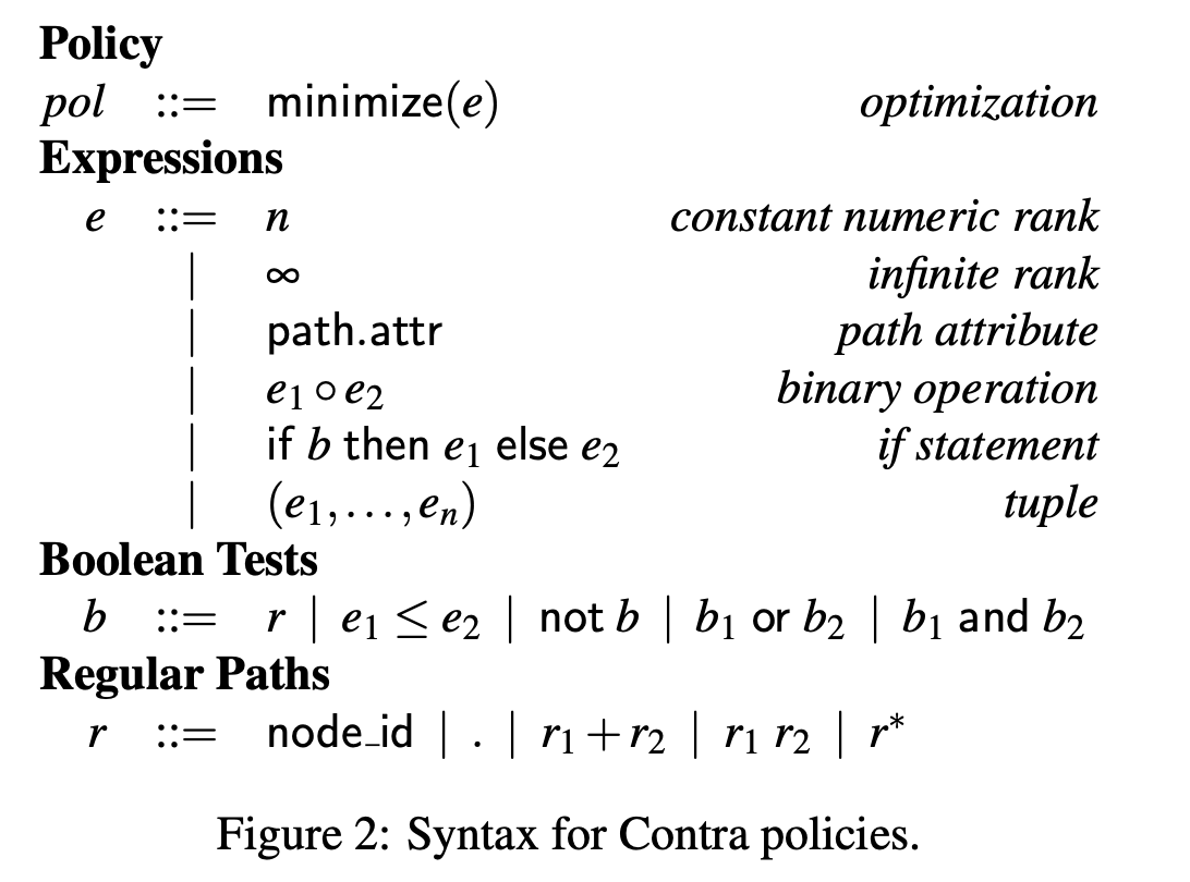
Sample language to map paths to ranks based on their performance
Policies

Widest Shortest Path: least utilized path among shortest paths
Source-local preference: regular expression to specify paths
Compilation using Merlin (a language for provisioning network resources)
-
Automata are generated from policies. (b)&(c)
-
Intermedia representation (product graph) is generated with automata, checked with actual topology (d)
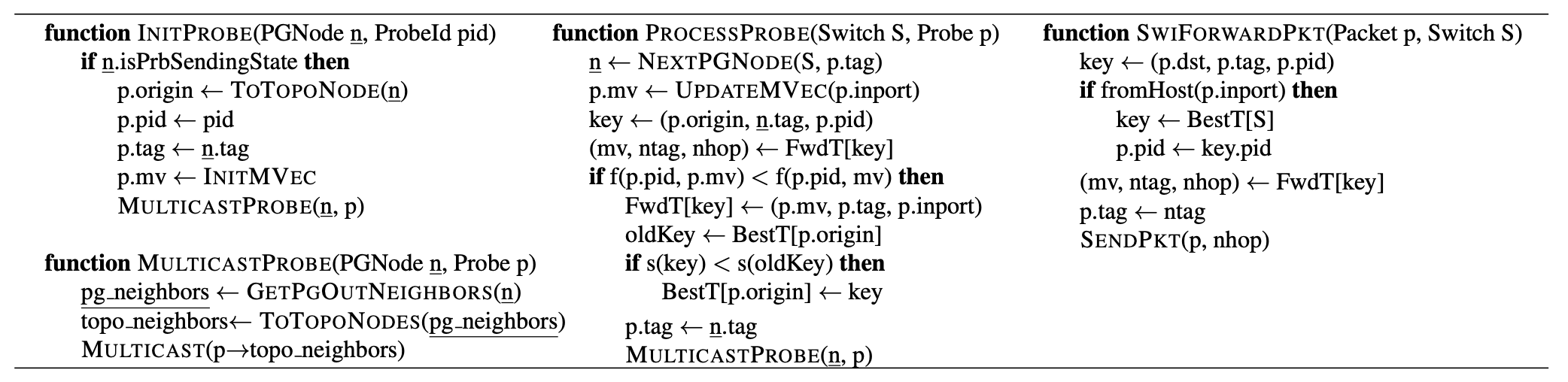
- forwarding tables are populated during runtime (e) when probes arrive carrying information on the pathway (metrics, next hop switch)
- Synthesize P4 programs to track policy states during runtime
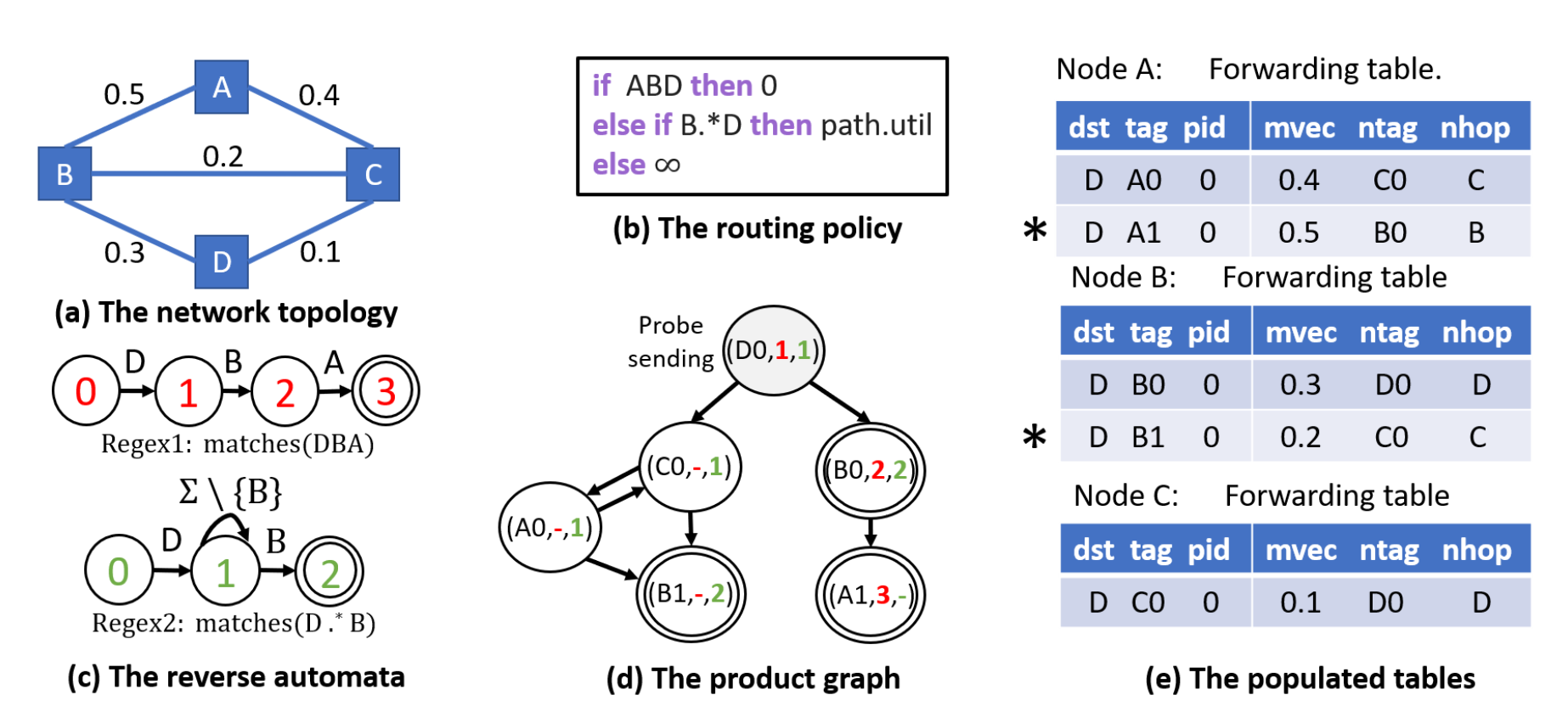
Product Graph
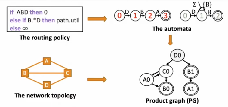
Policy -> automata + topology = Product Graph
Each PG edge is a policy-compliant path for the topology
Forwarding
Uses forwarding table populated by the probes and automata for forwarding decisions. Example 1, node B to D, can go B-D or B-C-D, because metric for B-C-D is 0.2 < 0.3 of B-D, selects B-C-D. Example 2, for node A, metric of A-B-D is larger, but the automata says if ABD then 0 < 0.4 of A-C-D, selects A-B-D.
Probes
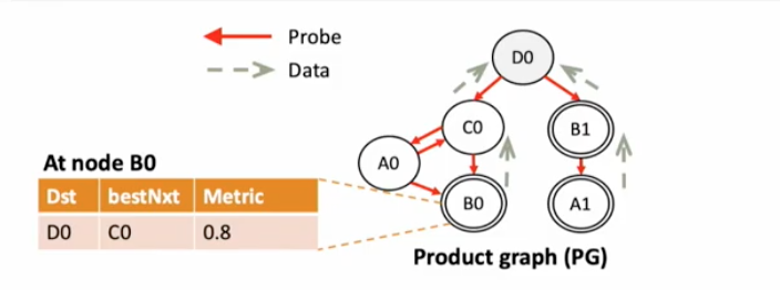
[D0 is a destination node, B0 and A1 are source nodes]
D0 initializes and sends probes with performance metrics, and the probes will be sent subsequently to the sources. Nodes along the way can know the path metrics based on information received and update forwarding table of its own and the probe to inform path condition change to its neighbors.
####Challenges:
- Transient loop in arbitrary topology: bc the algorithm is distance-vector + probes traversal takes time, asynchronous updates can cause loops (whereas fat-tree is tree-based, no loops by nature)
- See version number in probes to forced synchronization. e.g. probes 1 will not be used when probes 2 arrives regardless of their arrival time
- Probes cannot be sent too frequently as it will cause some nodes using newer probes, some use older probes. Limit probes sending rate to at least 0.5RTT to ensure old probes are propagated through whole pathway before sending new probes.
- Out-of-order delivery:
- Use flowlet switching to group packets in the same flow to avoid reordering at the receiver (work done by FLARE)
- Introduces looping because flowlet switching entries expire at different times, could form loops occasionally: count hops to monitor loops (distance-vector)
- Introduces policy violation because flowlet switching is constraint oblivious: add PG tags (policy) to flowlet entry so that flowlet becomes aware of the policy
- Constraint violation: because of loops + path metrics updates, could violate hard coded constraint (go through firewall…)
- Use Merlin to compute a product graph from automata (policies) and topology with probes and tags. In PG, tag represents the state of the automata (policy). At switch, tags will be checked to enforce global user policy.
Eval
Fat-tree topo:
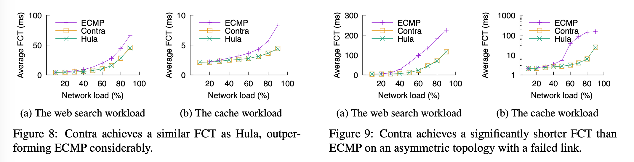
Fig8: symmetric fat-tree
Fig9: asymmetric fat-tree with failed link
metrics: FCT, task completion time
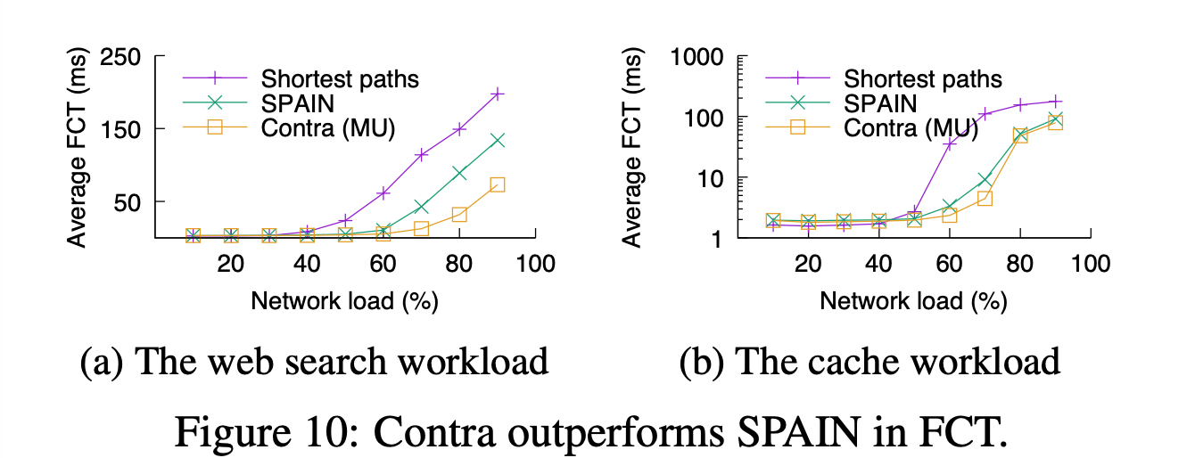
Arbitrary topo:
Hula/Conga will not work, beats SPAIN
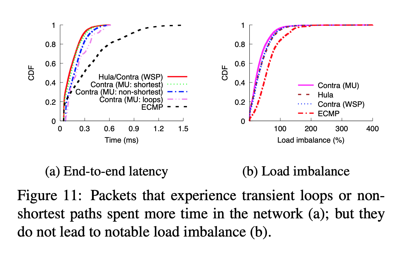
left = fast, up = more -> upleft means short latency
left = load balanced, up = more -> upleft means good balancing
10 Mar 2020
** This is a study & review of the Opera paper. I’m not an author.
SMORE: Semi-Oblivious Traffic Engineering Schema
Intro: Problems
- current TE focuses on performance or robustness, not both
- goal: good performance and failure tolerance.
- oblivious routing algorithm
- low-stretch, diverse, naturally load-balancing
- dynamically adjust sending rates
- combination is powerful and novel
FE System Study
-
FE components
- which path to take: path selection, slow -> infrequent
- how much traffic: rate adaptation, fast -> continuous
- challenge: to select small set of paths, to flexibly handle traffic scenarios.
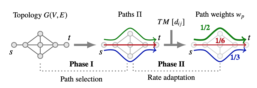
-
Path properties metrics
- low-stretch: low latency
- high diversity: good robustness
- good balancing: better performance
- good design needs to be capacity aware (not to over-utilize low-capacity links) & globally optimized (considers all pairs simultaneously)
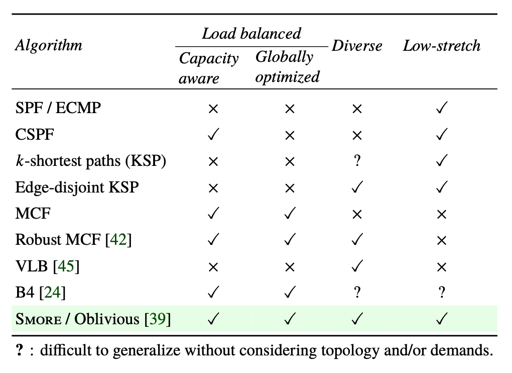
SMORE Design
-
Oblivious routing by Racke’s paper : a system of optional paths is chosen in advance for every source-destination pair, and every packet for that pair must travel along one of these optional paths, without consideration for demand.
- Why oblivious? To anticipate demands is challenging, and time consuming. Actual condition may differ a lot from anticipation. Avoids overfitting -> naturally robust.
- Routing tree / decomposition tree: In each iteration, algorithm generates a new routing tree with approximation algorithm –> low-stretch; updates weights of each link based on its capacity and cumulative utilization in the previous tree (penalize further use of already heavily utilized links) –> load-balancing; randomized intermediate destinations –> diversity.
-
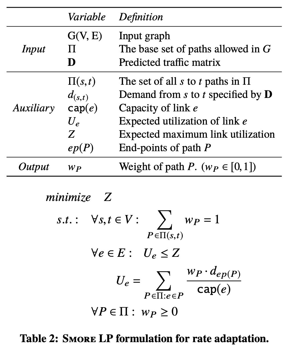
Rate Adaption: computes updated value of path weights by minimizing MLU (max link util) using a Linear Program, LP.
- paths are fixed –> LP computation is fast
Evaluation
Realistic simulation on Facebook’s backbone network carrying production traffic
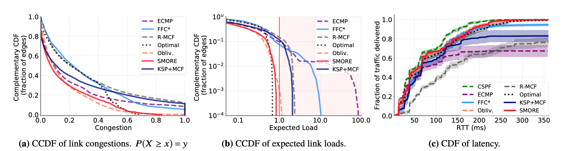
- lighter congestions
- no over-subscription for SMORE, whereas ECMP can over-subscribe 100X.
- latency is competitive with others
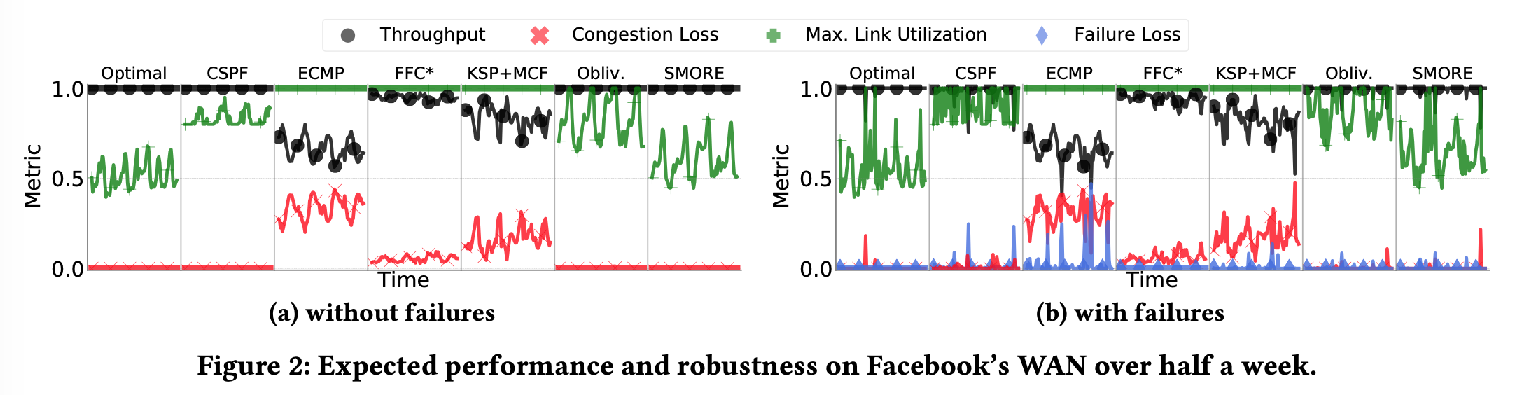
- SMORE overall
- low congestion loss (red → 0)
- high throughput (black → 1)
- (a) SMORE’s MLU performance (green) is greatly better other’s, and competitive to Optimal (using MCF, multi-commodity flow, to minimize MLU) which has the following cons:
- Solving MCF is slow thus limit responsiveness to changing demands. On average 25s for an optimized LP solver to solve MCF instances for a WAN.
- Small changes in TMs (traffic matrix) can lead to a significantly different solution to MCF, which leads to excessive routing churn.
- Ensuring continuous consistent updates to forwarding state at routers adds significant management complexity.
- (b) SMORE is also robust (tolerant to failures): failure losses (blue on the bottom next to zero) is minimal and stable
02 Mar 2020
** This is a study & review of the Opera paper. I’m not an author.
Opera: Expanding across time to deliver bandwidth efficiency and low latency
Abstract
Opera: dynamic network using multi-hop forwarding (expander-graph-based approach), but provides near-optimal bandwidth for bulk flows with direct forwarding overtime-varying source-to-destination circuits.
Key: rapid & deterministic reconfiguration of the network, so that at any time network implements an expander graph; across time, network provides bandwidth-efficient single-hop paths between all racks.
Intro
Reconfigurable networks aka dynamic network
Provision direct link between end points with high demand. Takes a long time to identify, reconfigure the network.
Problem: a trade-off between amortizing the overhead of reconfiguration against the inefficiency of sub-optimal configurations
Observation: most bytes in today’s datacenter networks are bulk traffic.
Goal: To minimize bandwidth tax paid by bulk traffic.
Solution: dynamic, circuit-switched topology, reconfigures small number of TOR switches uplinks, moving through a series of time-caring expander graphs.
Idea: this changing topology will ensure very pair of end points are allocated a direct link for bandwidth efficient connectivity for bulk traffic.
Challenge with Fat-tree: communication between racks has to go through intermediate switches, reduces network capacity between racks, thus Hadoop/MapReduce has “locality”
Expander topology: directly link an uplink of a TOR to other TORs (sparse graph, multiple short paths between source to destination) -> multiple hops of TOR to the destination TOR -> bandwidth waste -> establish single hop paths for source, destinations
Design
To find short path: expander graph, also fault-tolerant, because each pair has multiple paths.
To avoid bandwidth waste: reconfigure topology as needed, amortized costs very small for bulk traffic.
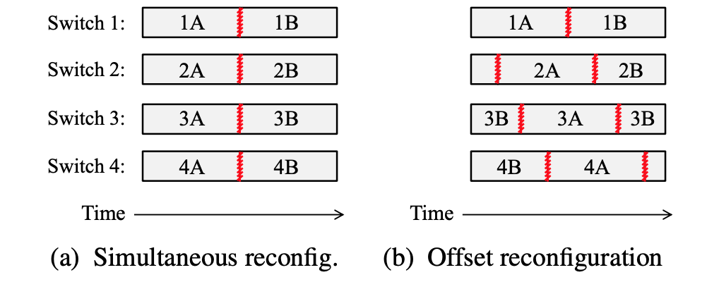
Staggered reconfiguration to ensure valid paths always exist. Continuous connectivity.
Expander graph: ensure 1. Multi hop path always exist. 2. Single hop path is provisioned. “Cycle time” is needed for each pair of source, destination to have a direct connection
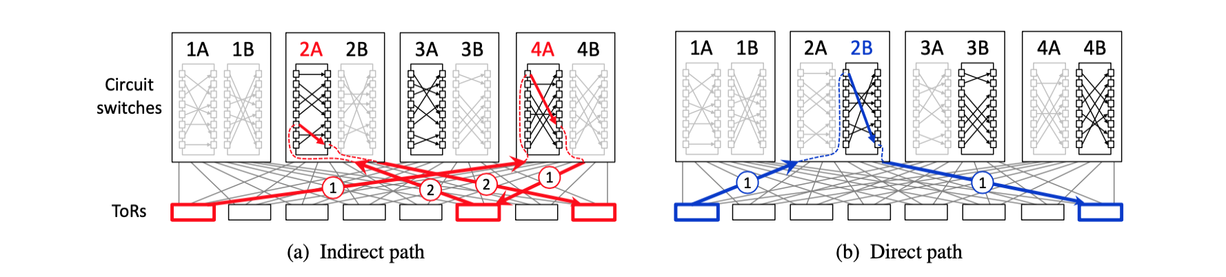
Example: Two-tier leaf-spine topology
Each TOR connects to the four circuit switches, and matching A is multi hop path for low-latency traffic, matching B is one-hop path for bulk traffic. Bulk traffic can wait until matching B is instantiated in switch 2 to begin transmission. Latency-sensitive data can immediately begin transmission with matching A.
Topology is generated before network operations (bootstrapping), no computation during operation.
Traffic size to determine using indirect path or waiting for direct path. Or to use application data to determine which one to use.
Eval
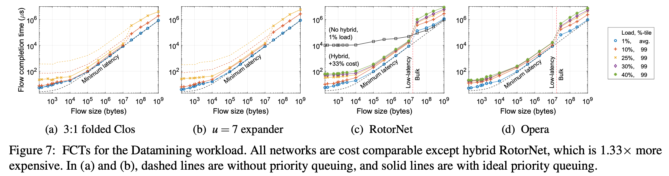
Opera outperform others, lower flow completion time, in law-latency traffic and build traffic.
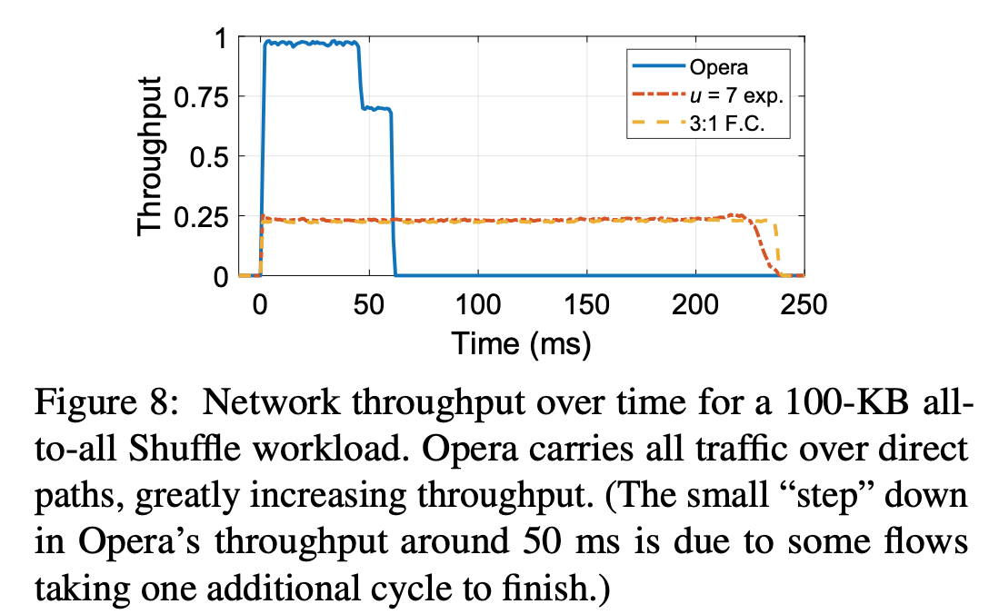
Opera is designed to handle bulk traffic with direct link, and this graph shows that Opera can achieve higher throughput with direct path.
Conclusion
Opera is a topology that implements a series of time-varying expander graphs that support low-latency traffic, and when integrated over time, provide direct connections between all endpoints to deliver high throughput to bulk traffic.